2 Asking Good Questions: Research Design
2.1 The Experiment You Never Agreed To
In January 2012, roughly 689,000 Facebook users had their News Feeds quietly altered. For one week, some users saw fewer posts containing positive emotional words. Others saw fewer posts containing negative emotional words. The researchers, a team from Facebook’s Core Data Science group and Cornell University, wanted to know whether emotional content in a social media feed could influence a person’s own emotional state. They called it “emotional contagion.”
The results, published in the Proceedings of the National Academy of Sciences (PNAS) in June 2014, were modest. Users who saw fewer positive posts wrote slightly more negative posts themselves, and vice versa. The effect sizes were tiny. Under normal circumstances, a study with small effects and a narrow scope might have attracted a paragraph in a science news roundup and nothing more.
Instead, it became one of the most controversial research studies of the decade.
The problem was not the findings. The problem was the design.
Nearly 700,000 people had been enrolled in a psychological experiment without their knowledge. No one had asked them. No one had told them. No one had given them the option to say no. The researchers argued that Facebook’s Terms of Service, which users accept when they create an account, covered this kind of research. The Terms of Service did mention that Facebook might use data for “research.” But there is a wide gap between a company analyzing click patterns to improve ad targeting and a company deliberately manipulating what people see in order to study changes in their emotional state. Most people, when they click “I Agree” on a terms-of-service page, are not imagining that they have just consented to a mood manipulation experiment.
The backlash was swift and broad. Privacy advocates pointed out that the study lacked meaningful informed consent. Psychologists noted that the study would never have been approved by a standard university institutional review board (IRB) without explicit consent from participants. The editor of PNAS added an “editorial expression of concern” to the published paper, a rare step, acknowledging concerns about the ethical procedures. Cornell’s IRB, which had reviewed the project, had determined that its own review was not required because Facebook had collected the data, not the Cornell researchers. This interpretation struck many as a convenient loophole rather than a principled decision. In the years since, the U.S. Department of Health and Human Services updated the Common Rule (the federal regulations governing human subjects research), with revisions that took effect in 2018. Those revisions extended protections more clearly to research involving data collected by third parties. The Facebook study helped catalyze that conversation, though regulatory gaps between academic and corporate research settings remain an active area of debate.
What makes the Facebook study such a useful starting point for a chapter on research design is that it illustrates, in a single case, most of the principles we need to discuss. The researchers had a question. They chose a method to answer it. They selected a sample. They made decisions about what to manipulate, what to measure, and whom to include. And they made those decisions with insufficient attention to the people affected by them.
Good research design is about more than getting the right answer. It is about asking the right question, choosing the right approach, protecting the people involved, and being transparent about every decision along the way. This chapter covers how to do all of that.
2.2 Two Kinds of Studies
In Chapter 1, we introduced the distinction between observational studies and experiments. That distinction is so central to everything that follows in this book that we need to treat it in much greater depth here.
If you have taken a course in research methods, you may have encountered a different but related classification: studies are sometimes described as exploratory, descriptive, or causal. Exploratory studies aim to develop initial understanding of a phenomenon that has not been well studied; they generate questions rather than test them. Descriptive studies aim to characterize what exists: how common something is, how groups compare, what patterns are present. Causal studies ask whether one thing produces another.
These two frameworks are not in conflict. They operate at different levels. Exploratory and descriptive studies are almost always observational: the researcher is watching and measuring, not intervening. Causal studies are most credibly conducted as experiments, because only controlled manipulation with random assignment can rule out the alternative explanations that observational data leaves open. When you see the observational/experimental distinction in this chapter, you can read it as the methodological dimension of a question whose purpose might be descriptive or causal. Understanding both frameworks deepens your ability to evaluate what a study can and cannot claim.
2.2.1 Observational Studies
In an observational study, the researcher watches, measures, and records, but does not intervene. The world does what it does, and you take notes.
Consider a researcher who wants to understand the relationship between sleep and academic performance among college students. They survey 500 students, asking them how many hours of sleep they typically get per night and collecting their GPAs from university records. They then look at whether students who sleep more tend to have higher GPAs.
This is an observational study. The researcher did not assign anyone to a sleep schedule. They observed the students as they were and recorded the data.
Observational studies are everywhere. A hospital compares outcomes for patients who chose Surgery A versus Surgery B. An economist examines whether countries with higher minimum wages have lower poverty rates. A marketing analyst looks at whether customers who open promotional emails spend more than customers who do not. In each case, the researcher is observing existing differences between groups, not creating those differences.
The great advantage of observational studies is feasibility. They are often cheaper, faster, and more ethical than experiments. You cannot randomly assign people to smoke for 30 years to study the health effects of tobacco. You cannot randomly assign children to poverty to study its effects on brain development. You cannot randomly assign countries to adopt different trade policies. For many of the most important questions in medicine, social science, and policy, observational studies are the only realistic option.
The great disadvantage is that observational studies, on their own, cannot establish causation. We will spend a full section on why later in this chapter. For now, the short version is that when you observe a difference between two groups that already existed before you showed up, you cannot be sure whether the difference in outcomes is caused by the factor you are studying or by some other way in which the groups differ.
2.2.2 Experiments
In an experiment, the researcher intervenes. They do more than observe the world as it is. They change something and watch what happens.
The defining feature of a true experiment is that the researcher controls the assignment of treatments. In the simplest case, participants are divided into two groups. One group receives the treatment of interest (the treatment group), and the other does not (the control group). Then the researcher compares outcomes between the two groups.
Suppose our sleep researcher wanted to move beyond observation. They recruit 100 students and randomly assign 50 of them to a “sleep coaching” program designed to increase their nightly sleep by one hour. The other 50 receive no intervention. At the end of the semester, they compare the GPAs of the two groups.
This is an experiment. The researcher created the difference between the groups by assigning the treatment. They did not merely observe a pre-existing difference.
Randomization is the ingredient that makes experiments so powerful. When participants are randomly assigned to treatment and control groups, any pre-existing differences between participants (their motivation, prior academic performance, stress levels, coffee consumption, everything) get distributed roughly equally across both groups. This means that if the treatment group ends up with higher GPAs at the end of the study, the most plausible explanation is the treatment itself, because the groups were comparable in every other respect at the start.
This is a strong claim, and it has limits that we will discuss. But it is the foundational logic of experimental design, and it is why randomized controlled experiments are often called the “gold standard” for establishing cause and effect.
2.2.3 The Spectrum Between Observation and Experiment
The line between observational studies and experiments is clearer in textbooks than in practice. Real research often falls somewhere in between.
Quasi-experiments are studies where the researcher exploits a “natural” assignment to treatment and control groups that was not random in the strict sense but might be close enough to be useful. For example, when a state raises its minimum wage and a neighboring state does not, researchers can compare employment trends in the two states before and after the change. Nobody randomly assigned states to different minimum wage policies, but the comparison has some of the logic of an experiment. Economists call this a “natural experiment” or a “difference-in-differences” design.
A/B tests are experiments conducted in digital environments. When a tech company shows half its users a blue “Buy Now” button and the other half a green one, then compares click-through rates, that is a randomized experiment. The Facebook emotional contagion study was, structurally, an A/B test. The ethical problem was not the experimental design itself but the absence of informed consent.
Retrospective studies look backward in time, using existing records to study past events. A researcher might examine medical records to compare outcomes for patients who received different treatments years ago. These are observational studies, but they often feel like experiments because the treatments are well-defined. The crucial difference is that the researcher did not control who got which treatment, so confounding is a serious concern.
Understanding where a study falls on this spectrum is essential for knowing how much confidence to place in its conclusions.
The phrase “gold standard” for randomized controlled trials comes from medicine, where the randomized controlled trial has been the benchmark for evaluating treatments since the mid-twentieth century. The first widely recognized RCT was the 1948 British Medical Research Council trial of streptomycin for pulmonary tuberculosis, designed and led by Austin Bradford Hill. Before that, treatments were evaluated by clinical experience, case reports, and expert opinion, methods that sound reasonable but produced centuries of medical practices that ranged from useless to actively harmful. Bloodletting persisted for over 2,000 years in Western medicine partly because no one ran a controlled experiment to check whether it worked. Bradford Hill later articulated the criteria for causal inference from observational data that bear his name, discussed later in this chapter.
2.3 How to Choose Your Sample
We introduced sampling concepts in Chapter 1; here we examine them in the context of research design.
Imagine you want to know the average amount of student loan debt carried by undergraduates at a large university with 15,000 students. You cannot survey all 15,000. You need a sample. But which students should you include?
The answer to this question matters far more than most people realize. A badly chosen sample can produce results that are not merely imprecise but systematically wrong. And the way a sample goes wrong is often invisible in the final data, which makes it especially dangerous.
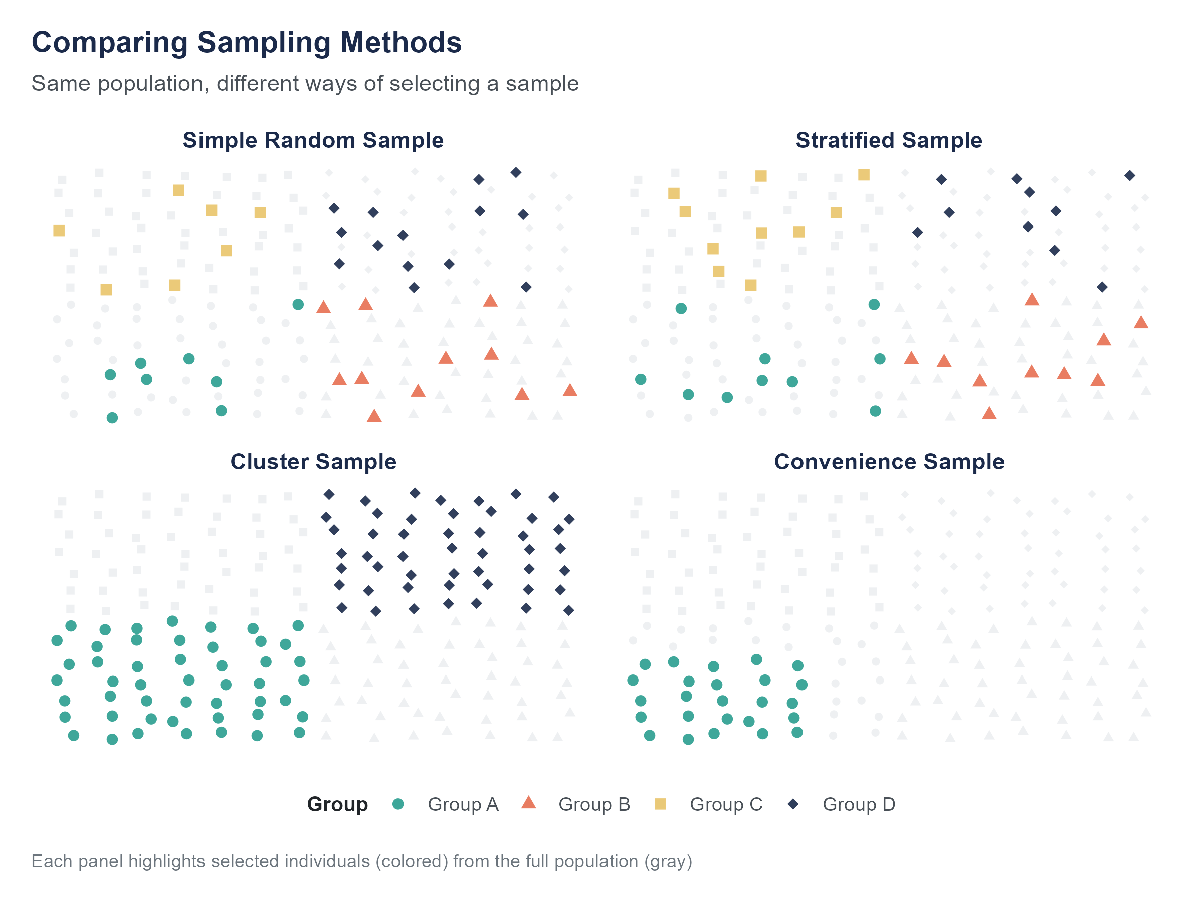
2.3.1 Simple Random Sampling
The most intuitive sampling method is the one you probably thought of first. Get a list of all 15,000 students, assign each one a number, and use a random number generator to select, say, 500 of them. Every student has an equal chance of being selected, and every possible sample of 500 students has an equal chance of being the one you draw.
This is simple random sampling, and it is the foundation on which most of the statistical methods in this book are built. When we talk about “random samples” without further qualification, this is what we mean.
Simple random sampling has a critical virtue. Because every member of the population has the same chance of being included, there is no systematic tendency for the sample to over-represent or under-represent any subgroup. Your sample might, by chance, include more seniors than freshmen, or more engineering majors than English majors. But there is no built-in bias pushing it in any particular direction. And as the sample gets larger, those random fluctuations shrink.
The practical challenge is that simple random sampling requires a complete list of the population, what statisticians call a sampling frame. For our student debt example, the university’s registrar presumably has such a list. But for many populations of interest, no such list exists. There is no master list of all Americans who have experienced food insecurity. There is no directory of every small business in the informal economy. When the sampling frame is incomplete or does not exist, simple random sampling is impossible, and researchers must get creative.
2.3.2 Stratified Sampling
Suppose you suspect that student loan debt varies a lot by class year, with seniors carrying more debt than freshmen simply because they have been borrowing longer. You want your sample to reflect the university’s distribution across class years. You could trust simple random sampling to give you roughly the right proportions, but with only 500 students, you might end up with too few freshmen or too many juniors by chance alone.
Stratified sampling solves this by dividing the population into non-overlapping subgroups (called strata) and then drawing a simple random sample from each stratum separately. The most common form draws from each stratum in proportion to its size in the population; this is called proportional stratified sampling. If the university is 30% freshmen, 25% sophomores, 25% juniors, and 20% seniors, you draw 150 freshmen, 125 sophomores, 125 juniors, and 100 seniors, giving you exactly 500. Now your sample is guaranteed to match the population’s composition by class year.
Stratification improves precision when the variable you stratify on is related to the variable you are measuring. If seniors do in fact carry more debt than freshmen, a stratified sample will give you a more accurate estimate of the overall average than a simple random sample of the same size, because you have eliminated one source of random variation.
You can stratify on more than one variable (for instance, class year and residency status, in-state vs. out-of-state), but the more strata you create, the more complex the logistics become. With four class years and two residency categories, you already have eight strata, and you need enough students in each one to produce reliable estimates.
When proportional stratified sampling gives you too few observations in a small but important subgroup, disproportional stratified sampling may be more appropriate. In this approach, you intentionally over-sample from smaller strata to ensure adequate representation. A study of religious discrimination in hiring might use proportional sampling for large groups but deliberately over-sample members of small religious minorities, who would otherwise appear in too few numbers for meaningful analysis. After data collection, the over-sampled groups are statistically weighted back to their true population proportions for any estimates about the population as a whole. This approach is common in studies of rare conditions, small demographic groups, and under-studied populations where proportional sampling would produce cells too thin to analyze.
2.3.3 Cluster Sampling
Now suppose you do not have a list of all 15,000 students but you do have a list of all 600 course sections offered this semester, and you know that virtually every student is enrolled in at least one course. You could randomly select 30 course sections and survey every student in those sections.
This is cluster sampling. Instead of sampling individuals directly, you sample naturally occurring groups (clusters) and then include all members of the selected clusters.
Cluster sampling is often used for practical reasons. It is easier to visit 30 classrooms than to track down 500 individual students scattered across campus. Public health surveys often use cluster sampling, randomly selecting neighborhoods or clinics and then surveying everyone at the selected sites.
The downside is that cluster sampling is generally less precise than simple random sampling or stratified sampling for a given sample size. People within the same cluster tend to be more similar to each other than to people in other clusters. Students in the same course section might be more similar in major, class year, and interests than a random cross-section of the university. This means each cluster gives you less new information than you would get from the same number of randomly selected individuals.
2.3.4 Systematic Sampling
There is one more common method worth knowing. Suppose you have a list of all 15,000 students sorted alphabetically and you want a sample of 500. You calculate that 15,000 divided by 500 equals 30. You pick a random starting point between 1 and 30, say student number 17, and then select every 30th student after that. Student 17, student 47, student 77, and so on.
This is systematic sampling. It is simple to implement and produces a sample that is spread evenly across the list. As long as the list itself does not have a hidden pattern that aligns with your sampling interval (which is rare but not impossible), systematic sampling works well in practice.
One risk arises when the list has a periodic structure. If a list of apartment units alternates between corner units and interior units, and your sampling interval happens to match that pattern, you could end up with a sample that is all corner units or all interior units. In practice this is unusual, but worth checking.
The Sampling Explorer lets you compare all four sampling methods side by side. Draw repeated samples using simple random, stratified, cluster, and systematic methods and watch how much the estimates vary across approaches. Try drawing 20 stratified samples and 20 simple random samples from the same population and compare how tightly the estimates cluster. The difference is immediate and visible.
2.3.5 Convenience Sampling and Its Problems
In practice, many studies use none of the methods described above. Instead, they rely on whoever is easy to reach, a practice called convenience sampling. A psychology professor studies the students in their introductory class. A political pollster surveys people who answer their phones. A health researcher recruits volunteers from a social media post.
Convenience samples are not inherently useless, but they are inherently limited. The people who are easy to reach are almost never representative of the broader population. Students in a psychology class are younger, more educated, and more likely to be from what researchers Henrich, Heine, and Norenzayan (2010) famously called WEIRD societies (Western, Educated, Industrialized, Rich, and Democratic), than the world population at large. Their widely cited paper in Behavioral and Brain Sciences argued that the overwhelming majority of published psychology research has been conducted on WEIRD participants, yet the resulting findings have routinely been described as universal features of human cognition, behavior, and social interaction. The implications are substantial. Findings about perception, memory, moral reasoning, social norms, and decision-making that appear stable and robust in Western undergraduate samples have, in many cases, not replicated in other cultural contexts, or have replicated only partially. If convenience sampling has systematically shaped a field’s knowledge base for decades, then our understanding of “what people do” may really be a description of “what a specific and unrepresentative slice of humanity does.” People who answer calls from unknown numbers differ from those who do not, though it is a distinction most of us have quietly settled for ourselves. Social media volunteers differ from people who are not on social media or who do not follow the researcher’s account.
The problem is not that convenience samples exist. Many valuable studies have used them. The problem arises when researchers draw conclusions about a broad population from a convenience sample without acknowledging the limitations. If your study participants are all undergraduates at a single university, your findings apply to undergraduates at that university. They may or may not generalize to other people, and claiming otherwise requires an argument, not an assumption.
Open the Sampling Explorer on the companion website. Start with samples of 10, then increase to 50, 100, and 500, and watch the spread of estimates shrink. Try setting the population to have a rare subgroup (say, 5% of the total) and see how small samples can miss it entirely while larger samples capture it reliably.
2.4 Bias: When Data Leads You Astray
The word “bias” has a casual meaning (prejudice, unfairness) and a technical one. In statistics, bias refers to a systematic tendency for a method to produce results that are consistently too high, too low, or skewed in some particular direction. A biased method does more than make random errors. It makes errors that lean in the same direction, again and again.
Random error is like a dartboard where your throws scatter around the bullseye. Sometimes you are high, sometimes low, sometimes left, sometimes right, but on average you are close to the center. Bias is like a dartboard where the sights are off. Every throw lands in the same wrong spot, and throwing more darts does not fix the problem.
This distinction matters because increasing your sample size fixes random error but does not fix bias. A survey that systematically misses low-income households does not become representative just because you survey more people. It becomes a larger, more confidently wrong dataset.
The Total Survey Error Explorer maps every error type covered in this section as a clickable taxonomy tree. Select any node to see its definition, a practitioner example, and mitigation strategies. Each error is tagged with whether increasing sample size actually reduces it, a direct illustration of the distinction between random and systematic error. Use the List View to search across error types, or test yourself with the eight-question Self-Check quiz.
2.4.1 Selection Bias
Selection bias occurs when the process of selecting participants produces a sample that differs systematically from the population. We touched on this in Chapter 1. Here we dig deeper.
One famous historical example is the 1936 Literary Digest presidential poll. The magazine mailed mock ballots to about 10 million people, drawing its list from telephone directories, automobile registration records, magazine subscriber lists, and club and association rosters. It received approximately 2.4 million responses, an enormous sample by any standard. Based on those responses, the Literary Digest predicted that Alf Landon would defeat Franklin Roosevelt in a landslide, with Landon taking 57% of the popular vote. Roosevelt won 46 of 48 states, capturing approximately 61% of the vote.
What went wrong? Two problems compounded each other. First, the mailing list skewed heavily toward wealthier Americans: in 1936, during the Great Depression, telephones, cars, club memberships, and magazine subscriptions were all markers of relative affluence, and wealthier voters tended to favor Landon. But modern scholarship, notably Squire (1988), has established that this sampling bias alone cannot fully explain the magnitude of the error. The second and arguably more important problem was non-response bias. Of the 10 million ballots mailed, only about 24% came back. Landon supporters, more motivated by opposition to Roosevelt’s New Deal, were far more likely to return their ballots. Roosevelt’s supporters, who formed the larger share of the population, responded at much lower rates. The result was not merely a biased sample, it was a biased sample further filtered by differential non-response, compounding the original error. Meanwhile, George Gallup, using a much smaller but more carefully selected sample of about 50,000, correctly predicted Roosevelt’s victory.
The lesson has not been fully learned. In 2016, many polls underestimated support for Donald Trump in key states, partly because their samples underrepresented voters without college degrees, a group that broke heavily for Trump. The problem was not sample size. National polls surveyed thousands of people. The problem was that the samples did not accurately reflect the composition of the electorate.
Selection bias can also emerge from the way data is generated. Hospital data contains information only about people who went to the hospital, which means it misses everyone who was sick but did not seek treatment. Online product reviews come from people motivated enough to write a review, who tend to be either very satisfied or very dissatisfied. Crime statistics reflect crimes that were reported, investigated, and documented, which may differ from the actual incidence of crime in ways that correlate with race, geography, and policing practices.
2.4.2 Response Bias
Even when you have a good sample, the answers people give may not be accurate. Response bias occurs when respondents systematically give answers that deviate from the truth.
People tend to over-report behaviors they consider socially desirable (exercising, voting, flossing) and under-report behaviors they consider undesirable (drinking, drug use, prejudice). This is called social desirability bias, and it affects self-reported data of all kinds.
The way a question is worded can also introduce bias. In a classic demonstration, Loftus and Palmer (1974) found that people estimated higher vehicle speeds when asked “How fast were the cars going when they smashed into each other?” compared to “How fast were the cars going when they contacted each other?”, a difference of roughly 9 miles per hour on average (40.5 mph versus 31.8 mph), despite participants watching the same footage. Same event, different wording, different answers.
Leading questions, loaded terms, question order, and even the visual layout of a survey can all shape responses. A survey that asks “Do you support raising taxes to fund early childhood education?” will get different results than one that asks “Do you support raising taxes?” followed by a separate question about early childhood education. The survey designer’s choices are baked into the data, often invisibly.
2.4.3 Non-Response Bias
You mail out 1,000 surveys and get 200 back. Your response rate is 20%. The question that should keep you up at night is whether the 800 people who did not respond are different from the 200 who did.
Non-response bias occurs when the people who choose not to participate are systematically different from those who do. If dissatisfied customers are less likely to respond to a satisfaction survey (perhaps because they have already left), your results will overestimate satisfaction. If healthier people are more likely to participate in a health study (because they have the time and energy), your results will overestimate the health of the population.
Non-response bias has gotten worse over time as survey response rates have declined. In the 1970s, telephone surveys routinely achieved response rates of 70% or higher. Today, rates below 10% are common for cold-call surveys. When nine out of ten people decline to participate, the assumption that respondents represent the broader population becomes very hard to defend.
Researchers address non-response bias through follow-up contacts, incentive payments, and statistical weighting, adjusting the results to account for known differences between respondents and the population. None of these solutions is perfect, and all of them require assumptions about why people did or did not respond.
2.4.4 Survivorship Bias
During World War II, the U.S. military studied bombers that returned from combat missions to figure out where to add armor. The planes that came back had bullet holes concentrated in certain areas: the fuselage, the wings, the fuel system. The initial inclination was to reinforce those areas.
Abraham Wald, a mathematician working with the Statistical Research Group at Columbia University, pointed out the flaw in this reasoning. The military was only seeing the planes that had survived. The planes hit in the engines or cockpit had not made it back. The bullet holes on the surviving planes showed where a plane could afford to be hit. The missing data (the planes that did not return) indicated where the armor was actually needed. Wald’s analysis, documented in a 1943 memorandum, redirected attention to the unobserved cases rather than the observed ones.
This is survivorship bias: the error of drawing conclusions from a sample that has been filtered by a survival process, while ignoring the cases that did not survive the filter. (Chapter 1 briefly noted this concept and the Wald example; here we treat it in full.)
Survivorship bias appears in many contexts. Business books study successful companies and extract lessons, without accounting for how many companies followed the same practices and failed. We read about college dropouts who became billionaires without accounting for the far larger number of dropouts who did not. Mutual fund performance statistics can appear impressive partly because funds that perform badly get closed and disappear from the database, a phenomenon that inflates apparent average returns.
The antidote to survivorship bias is to ask a specific question about every dataset you encounter. Who or what is missing from this data, and why?
Abraham Wald’s work on survivorship bias during World War II is one of statistics’ most celebrated examples, but Wald himself was far more than this single insight. Born in 1902 in Cluj, then part of the Austro-Hungarian Empire (present-day Romania), Wald was a Jewish mathematician who fled to the United States after the Nazi annexation of Austria in March 1938. At Columbia, he produced foundational work in statistical decision theory and sequential analysis, the latter allowing researchers to analyze data as it accumulates rather than waiting for a predetermined sample size. This work remains central to how clinical trials are monitored today. Wald died in a plane crash in southern India in December 1950, at the age of 48.
2.6 When Can We Claim Causation?
Given everything we have discussed, when is it legitimate to say that X causes Y? This is a question we will revisit in later chapters, especially when we cover regression, but it is worth laying the groundwork now.
2.6.1 The Experimental Path
The most straightforward path to a causal claim is a well-designed randomized experiment. At its core, establishing causation requires three things. First, there must be a demonstrated relationship between the variables: X and Y must co-vary, meaning changes in X are associated with changes in Y. This is sometimes called concomitant variation. Second, the cause must precede the effect; X must come before Y in time. Third, the relationship must survive the elimination of alternative explanations: other variables that could plausibly produce the observed pattern must be ruled out.
In a well-designed experiment, all three conditions can be satisfied together. Random assignment creates the association, the manipulation establishes the time order, and the comparison between groups allows you to rule out alternatives. The strongest experiments also incorporate the following features.
A control group provides a baseline: without it, you cannot know whether the outcome changed because of the treatment or because of something else that happened during the study period.
Blinding prevents expectations from influencing results. When possible, participants do not know whether they are in the treatment or control group (single-blind), and neither do the researchers who assess outcomes (double-blind). Without blinding, knowing one’s group assignment can change behavior in ways that contaminate the comparison.
Replication across multiple studies, ideally by different researchers in different settings, is what transforms a single finding into scientific consensus. The history of psychology offers many cautionary tales of effects that failed to replicate, so convergence across independent studies matters.
When all of these conditions are met, a causal claim is on strong footing. Few studies satisfy every condition perfectly, so the strength of a causal claim is always a matter of degree.
2.6.2 The Observational Path
For many important questions, experiments are not feasible. You cannot randomly assign people to smoke, to grow up in poverty, or to live in neighborhoods with different levels of air pollution. Does that mean we can never make causal claims about the effects of smoking, poverty, or pollution?
In practice, the scientific community does make causal claims based on observational data, but the bar is higher. The most famous example is smoking and lung cancer. The evidence that smoking causes cancer is overwhelming, but it comes almost entirely from observational studies. No randomized experiment has ever assigned humans to smoke for decades.
The case for causation from observational data typically rests on several converging lines of evidence, articulated by epidemiologist Sir Austin Bradford Hill in a 1965 lecture. The criteria that bear his name include the following considerations.
Consistency. The association has been found across multiple studies, in different populations, using different methods.
Strength. The association is large. Smokers are not 5% more likely to develop lung cancer. They are 15 to 30 times more likely, depending on the amount smoked.
Dose-response relationship. More exposure is associated with more effect. Heavier smokers develop cancer at higher rates than lighter smokers.
Temporal ordering. The cause precedes the effect. Smoking comes before cancer, not the other way around.
Biological plausibility. There is a credible mechanism. We understand how carcinogens in tobacco smoke damage lung tissue.
Elimination of alternative explanations. (This is a summarizing principle rather than one of Hill’s original nine named criteria.) Known confounders have been accounted for, and the association persists.
These criteria are guidelines rather than a checklist. No single criterion is necessary or sufficient. But the more of them that are satisfied, the stronger the case for causation.
We will return to these ideas in Chapters 10 and 11, where regression models provide tools for statistically controlling for confounders. For now, the takeaway is this: experiments are the most direct route to causal claims. Observational studies can support causal claims when the evidence is strong, consistent, and resistant to alternative explanations. And a single observational study, no matter how large, is rarely enough on its own.
2.7 The Ethics of Research Design
The Facebook study was not the first time researchers caused harm by treating research design as a purely technical exercise. It was not even the worst case. But it serves as a useful anchor for a conversation about ethics that runs through every stage of the research process.
2.7.1 Informed Consent
The principle of informed consent means that people who participate in research should know they are participating, understand what the research involves, understand any risks, and have the genuine ability to decline without penalty.
This principle did not emerge from abstract philosophizing. It emerged from horror. The Nuremberg Code of 1947 was written in response to the medical experiments conducted by Nazi physicians on concentration camp prisoners during World War II. The Declaration of Helsinki, first adopted in 1964 by the World Medical Association and revised multiple times since, extended and formalized these protections specifically for medical research involving human participants. The Belmont Report, published in 1979 by the U.S. National Commission for the Protection of Human Subjects of Biomedical and Behavioral Research, established the ethical framework that governs research in the United States to this day, built on three principles: respect for persons, beneficence, and justice.
In the Facebook study, informed consent was essentially absent. The researchers argued that the Terms of Service constituted consent, but terms of service are legal documents designed to protect the company, not research protocols designed to protect participants. Millions of people accept terms of service without reading them. Even among those who read them, very few would understand that they were consenting to participation in a psychological experiment.
The standard for informed consent in research is higher than the standard for agreeing to a commercial contract, and it should be. Research participants are not customers making a purchasing decision. They are people whose data, behavior, or bodies are being used to generate knowledge, often for the benefit of others. They deserve to know what they are contributing to and to have a real choice about whether to contribute.
2.7.2 Power and Data Collection
Who gets studied, and who does the studying? These questions sit at the center of an established body of scholarship in research ethics, feminist science studies, and critical data studies, not a peripheral concern but a recognized analytical framework for understanding how power shapes what knowledge gets produced.
The language we use in research reflects these power dynamics. For decades, people enrolled in studies were routinely called “subjects,” a word that carries an implicit relationship of authority over the studied person. The preferred term today is participant, which recognizes that people who take part in research have agency and rights, not just compliance and obligations. The shift in language is not cosmetic. It reflects a genuine shift in how the research community understands the relationship between researchers and the people they study.
In their book Data Feminism, Catherine D’Ignazio and Lauren Klein argue that data science (broadly, the practice of extracting knowledge and insight from data using statistical, computational, and domain expertise) is not neutral. The choices about what to measure, what categories to use, whose perspectives to center, and whose to ignore are shaped by the power structures of the institutions that collect and analyze data. A dataset is not a mirror of reality. It is a product of decisions, and those decisions reflect who had the power to make them. As they put it, in data work as in other domains, power imbalances shape what questions get asked, who gets to ask them, and whose lives become the data.
Cathy O’Neil’s Weapons of Math Destruction (2016) documents how this plays out in practice. Algorithms used for hiring, lending, college admissions, and criminal sentencing can systematically disadvantage the communities that have the least power to contest or even detect their operation, often while appearing to be objective because they are mathematical. The appearance of neutrality can obscure embedded bias in ways that human decision-makers’ biases cannot, precisely because the process is opaque.
Consider the case of Henrietta Lacks, an African American woman whose cancer cells were taken during a biopsy at Johns Hopkins Hospital in 1951 without her knowledge or consent. Those cells, known as HeLa cells, became one of the most important tools in medical research, contributing to developments in cancer treatment, vaccine development, virology, and genetics. The Lacks family did not learn about the cells until decades later and received no compensation while companies commercialized products developed using her tissue. The story, documented in Rebecca Skloot’s The Immortal Life of Henrietta Lacks (2010), illustrates how race, class, and institutional power shaped who was treated as a research participant and on whose terms.
The collection of data from marginalized communities without their consent or benefit is not only a historical issue. Joy Buolamwini and Timnit Gebru’s 2018 research, published as “Gender Shades” in the Proceedings of Machine Learning Research, demonstrated that commercial facial recognition systems performed substantially worse on darker-skinned faces than on lighter-skinned faces, with error rates for darker-skinned women up to 34 percentage points higher than for lighter-skinned men. Predictive policing algorithms trained on historical arrest data, which reflects decades of racially biased policing practices, produce outputs that concentrate police attention in communities of color, creating a self-reinforcing cycle. Data reflects the world that generated it, including the injustices in that world. Analyzing that data without acknowledging those injustices can reinforce them.
In 2016, the investigative journalism team at ProPublica (Julia Angwin, Jeff Larson, Surya Mattu, and Lauren Kirchner) published an analysis of COMPAS (Correctional Offender Management Profiling for Alternative Sanctions), a commercial risk assessment algorithm used across the United States to predict whether a defendant would re-offend before trial or sentencing. Their analysis found that the algorithm was roughly equally accurate overall for Black and white defendants, but the types of errors it made differed systematically. Black defendants who did not go on to re-offend were almost twice as likely as white defendants to be incorrectly classified as high risk. White defendants who did re-offend were more likely to be incorrectly classified as low risk. The company that produced COMPAS argued that its algorithm satisfied one established definition of fairness: equal predictive accuracy across groups. ProPublica argued that it violated another: equal false positive rates across groups. Subsequent academic research has established that these two definitions of fairness are mathematically incompatible: no algorithm can simultaneously satisfy both when base rates differ across groups. This means “fairness” in algorithmic systems is not a technical problem with a single correct solution. It is an ethical and political question about which errors matter more and who bears their cost, questions that statistics can illuminate but cannot resolve. For the original analysis, see “Machine Bias” at propublica.org.
2.7.3 Ethical Obligations at Every Stage
Ethics is not a box you check at the beginning of a study and then forget about. Ethical considerations arise at every stage of research design.
In choosing a question. Whose questions get asked? Whose problems get studied? When data science resources (defined earlier in this chapter) flow disproportionately toward problems that interest wealthy institutions, the problems of less powerful communities go unexamined.
In designing the study. Who is included and who is excluded? What categories are offered on a survey? If a survey asks about gender with only “male” and “female” as options, it erases non-binary respondents. If a clinical trial excludes pregnant women “for safety,” it means that drugs reach the market without evidence about their effects during pregnancy.
In collecting data. Are participants fully informed? Do they have actual power to decline? A worker asked to participate in a company-sponsored study may feel pressured even if participation is technically voluntary. A student asked by a professor to fill out a survey may worry about consequences for declining.
In analyzing data. Are the researchers transparent about their methods? Do they report results that are inconvenient for their hypothesis, or do they selectively present only the findings that tell the story they want? This is a form of bias that no sampling method can fix.
In reporting results. Who has access to the findings? Are the results communicated in ways that people can actually understand and use? Publishing a finding in an academic journal behind a paywall serves a very different constituency than making it available to the community that was studied.
D’Ignazio and Klein’s Data Feminism (MIT Press, 2020) is available as an open-access book at data-feminism.mitpress.mit.edu and provides a thorough, readable treatment of these themes. It is worth engaging with in full, not because it provides easy answers, but because it provides better questions.
Ask an AI tool to summarize a research study and it will almost always give you a confident answer. What it will rarely do, unless you ask, is tell you whether the study was observational or experimental, and what that distinction means for the conclusions.
This matters because AI tools routinely describe observational findings using causal language. “Researchers found that coffee reduces the risk of heart disease” is how an AI might summarize a study that actually found an association between coffee consumption and lower heart disease rates in a cohort of volunteers. The study did not manipulate coffee intake. It did not randomly assign anyone to drink or abstain. It cannot support the claim that coffee reduces anything. But the AI summary sounds like it can, because the AI does not distinguish between “is associated with” and “causes.”
The same problem extends to confounders. If you ask an AI to identify the key findings of a study, it will report the results as stated. It will not, on its own, ask whether important confounders were measured, whether the comparison groups were comparable, or whether the sampling method limits generalizability. These are the questions this chapter has trained you to ask, and they are precisely the questions that AI tools skip.
When you use AI to help you read or summarize research, always follow up with three questions: Was this study observational or experimental? What confounders might explain the result? How was the sample selected? If the AI’s summary does not address these, the summary is incomplete regardless of how polished it sounds.
2.8 Putting It All Together: Evaluating a Study
When you encounter a research study (whether in a news article, a journal paper, or a business report), here is a framework for evaluating its design.
1. What is the research question? Is it clearly stated? Is it a question that data can actually answer?
2. Is it observational or experimental? If observational, be cautious about causal claims. If experimental, check whether randomization was used and whether there was a proper control group.
3. How was the sample selected? Was it a probability sample (simple random, stratified, cluster, systematic) or a convenience sample? Does the sampling frame match the population of interest?
4. How large is the sample? Larger samples give more precise estimates, but size alone does not fix bias. A biased sample of 10,000 is worse than an unbiased sample of 500.
5. What biases might be present? Think about selection bias, response bias, non-response bias, and survivorship bias. Consider who might be missing from the data and why.
6. What confounders might exist? If the study claims an association between two variables, think about what third variables could be creating or inflating that association.
7. Were ethical standards followed? Did participants give informed consent? Were vulnerable populations protected? Is the data being used in ways participants would reasonably expect?
8. Are the conclusions proportional to the evidence? A well-designed randomized experiment can support stronger conclusions than an observational study. A single study, no matter how well designed, provides weaker evidence than multiple studies with consistent findings.
This framework is not a formula. It is a habit of mind. The more you practice it, the better you will become at distinguishing studies that deserve your trust from studies that do not.
2.9 Looking Ahead
In Chapters 3 and 4, we will turn to the tools for describing what is in a dataset, using numbers and pictures. These tools may seem simpler than research design, but they depend on everything we have covered here. A beautiful histogram of a biased sample is still a picture of bias. A summary statistic calculated from confounded data summarizes the wrong thing. The methods in the next chapters are powerful, but only when applied to data that was collected thoughtfully.
Research design is not the glamorous part of statistics. It does not involve elegant formulas or impressive software. But it is the part that determines whether your analysis means anything at all.
2.10 Key Terms
- Observational study: A study in which the researcher observes and measures without intervening or assigning treatments.
- Experiment: A study in which the researcher deliberately assigns treatments to participants and compares outcomes.
- Randomized controlled experiment: An experiment in which participants are randomly assigned to treatment and control groups, considered the strongest design for establishing cause and effect.
- Quasi-experiment: A study that resembles an experiment but lacks true random assignment, often exploiting natural or policy-driven variation.
- A/B test: A randomized experiment, typically conducted in a digital environment, comparing two versions of something (a webpage, an email, an ad) to see which performs better.
- Treatment group: The group in an experiment that receives the intervention being studied.
- Control group: The group in an experiment that does not receive the intervention, serving as a baseline for comparison.
- Blinding: A design feature in which participants (single-blind) or both participants and researchers (double-blind) do not know who is in the treatment or control group.
- Simple random sampling: A sampling method in which every member of the population has an equal chance of being selected.
- Sampling frame: A complete list of the population from which a sample is drawn.
- Stratified sampling: A sampling method that divides the population into non-overlapping subgroups (strata) and samples from each stratum separately.
- Cluster sampling: A sampling method that randomly selects groups (clusters) from the population and includes all members of the selected clusters.
- Systematic sampling: A sampling method that selects every kth member from a list, starting at a randomly chosen point.
- Convenience sampling: A non-probability sampling method that uses whoever is easiest to reach.
- Bias: A systematic tendency for a method to produce results that deviate from the truth in a consistent direction.
- Selection bias: Bias arising from the way participants are chosen for a study, producing a sample that does not represent the population.
- Response bias: Bias arising from participants giving inaccurate answers, often due to social desirability, question wording, or question order.
- Non-response bias: Bias arising when people who do not participate in a study are systematically different from those who do.
- Survivorship bias: Bias arising from studying only the cases that passed through some selection or survival process, while ignoring those that did not.
- Social desirability bias: A specific form of response bias in which respondents over-report socially approved behaviors and under-report disapproved ones.
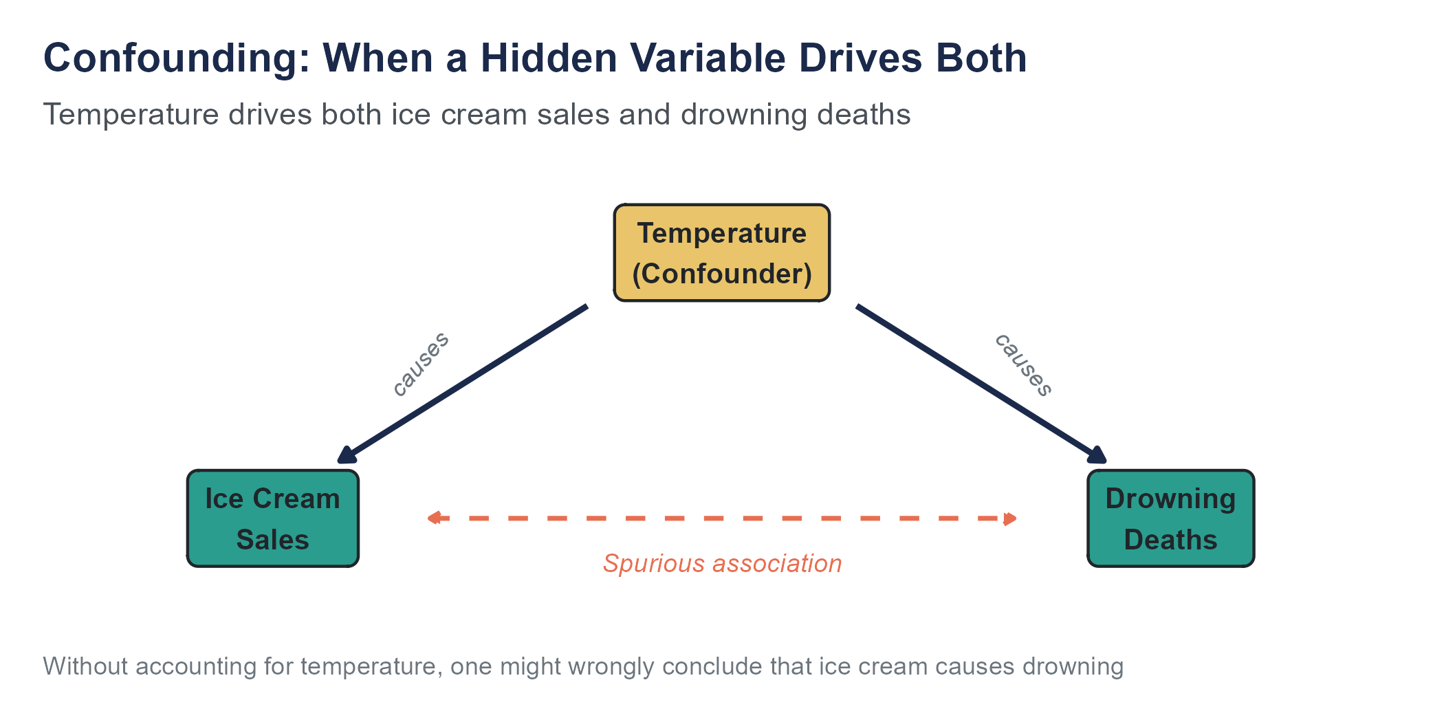
- Confounding variable (confounder): A variable that influences both the explanatory variable and the response variable, creating a misleading association between them.
- Lurking variable: Another term for a confounding variable, emphasizing that it may not be measured or even recognized.
- Simpson’s paradox: A phenomenon in which a trend that appears in aggregated data reverses or disappears when the data is separated into subgroups.
- Informed consent: The principle that research participants should understand what a study involves, including any risks, and should freely agree to participate.
- Institutional review board (IRB): A committee that reviews research proposals to ensure they meet ethical standards for the protection of human participants.
- Bradford Hill criteria: A set of guidelines, articulated by epidemiologist Sir Austin Bradford Hill in 1965, for evaluating whether an observed association in observational data is likely to be causal.
- Concomitant variation: The condition that cause and effect must co-vary: changes in the explanatory variable must be associated with changes in the outcome variable.
- Explanatory variable: The variable hypothesized to influence or predict the response. Also called the independent variable or predictor.
- Randomization: The process of using chance to assign participants to treatment and control groups, ensuring that pre-existing differences are approximately balanced.
- Response variable: The variable being studied as the outcome. Also called the dependent variable.
- Retrospective study: A study that looks backward in time, using existing records or recall to reconstruct what happened to participants.
2.11 Further Reading and References
The following works are cited in this chapter or provide valuable additional context for the ideas covered here.
On the Facebook emotional contagion study: Kramer, A. D. I., Guillory, J. E., & Hancock, J. T. (2014). Experimental evidence of massive-scale emotional contagion through social networks. Proceedings of the National Academy of Sciences, 111(24), 8788–8790.
On WEIRD sampling and its consequences: Henrich, J., Heine, S. J., & Norenzayan, A. (2010). The weirdest people in the world? Behavioral and Brain Sciences, 33(2–3), 61–83.
On the Literary Digest poll: Squire, P. (1988). Why the 1936 Literary Digest poll failed. Public Opinion Quarterly, 52(1), 125–133.
On response bias and eyewitness testimony: Loftus, E. F., & Palmer, J. C. (1974). Reconstruction of automobile destruction: An example of the interaction between language and memory. Journal of Verbal Learning and Verbal Behavior, 13(5), 585–589.
On research ethics and the Belmont Report: National Commission for the Protection of Human Subjects of Biomedical and Behavioral Research. (1979). The Belmont Report. U.S. Department of Health, Education, and Welfare.
On power, data, and algorithmic bias: D’Ignazio, C., & Klein, L. F. (2020). Data feminism. MIT Press. Available open access at data-feminism.mitpress.mit.edu.
O’Neil, C. (2016). Weapons of math destruction: How big data increases inequality and threatens democracy. Crown.
ProPublica. (2016). Machine bias: There’s software used across the country to predict future criminals. And it’s biased against blacks. Angwin, J., Larson, J., Mattu, S., & Kirchner, L. propublica.org/article/machine-bias-risk-assessments-in-criminal-sentencing.
On Henrietta Lacks: Skloot, R. (2010). The immortal life of Henrietta Lacks. Crown.
On facial recognition bias: Buolamwini, J., & Gebru, T. (2018). Gender shades: Intersectional accuracy disparities in commercial gender classification. Proceedings of Machine Learning Research, 81, 1–15.
On the Bradford Hill criteria: Hill, A. B. (1965). The environment and disease: Association or causation? Proceedings of the Royal Society of Medicine, 58(5), 295–300. (The lecture that introduced the nine criteria for evaluating causal claims from observational data, discussed in this chapter’s section on when observational evidence can support causation.)
A full R walkthrough of this chapter is online at stats.marginoferrormedia.com/walkthroughs/r-ch02.html. It simulates simple random, stratified, cluster, and systematic sampling on a 200-student population, plus a sample-size stability simulation.
2.12 Exercises
2.12.1 Check Your Understanding
In the Facebook emotional contagion study, researchers manipulated users’ News Feeds and measured changes in the emotional tone of their posts. Was this an observational study or an experiment? Explain your reasoning.
A school district wants to know whether a new math curriculum improves test scores. They implement the new curriculum at five schools and keep the old curriculum at five other schools, then compare end-of-year test scores. Is this an experiment or an observational study? If it is an experiment, is it a randomized experiment? What concerns might you have about this design?
Explain the difference between stratified sampling and cluster sampling. In stratified sampling, you sample from each subgroup. In cluster sampling, you sample entire subgroups. Why does this distinction affect the precision of your estimates?
A researcher surveys 1,000 adults by calling landline phones between 9 a.m. and 5 p.m. on weekdays. Identify at least two sources of bias in this sampling approach and explain the direction in which each bias would likely push the results.
A news article reports that children who eat dinner with their families at least five nights per week have higher grades than children who eat family dinners less often. A parent reads this and concludes that making their family eat dinner together will improve their child’s grades. What is the problem with this reasoning? Identify at least one plausible confounding variable.
Explain the difference between random sampling and random assignment. Which one helps with generalizability (applying results to the broader population)? Which one helps with establishing causation?
A fitness app reports that its users lose an average of 12 pounds in the first three months. Why might this statistic be misleading? Identify the specific type of bias most likely at work.
In your own words, explain why increasing the sample size reduces random error but does not reduce bias. Use an analogy or example.
A pharmaceutical company tests a new drug by giving it to 500 volunteers who responded to an advertisement and comparing their outcomes to published data on patients with the same condition who did not receive the drug. Identify at least two problems with this design.
Describe a scenario in which a quasi-experiment might be used because a true randomized experiment would be impractical or unethical. Explain what makes the study quasi-experimental rather than a true experiment.
2.12.2 Apply It
You want to estimate the average commute time for employees at a company with 2,000 workers spread across four office locations (New York with 800 employees, Chicago with 500, Denver with 400, and Atlanta with 300). Design a stratified sampling plan with a total sample of 200 employees. How many employees would you sample from each location? Why is stratified sampling preferable to simple random sampling here?
A university wants to survey students about their experience with mental health services on campus. They have a list of all 12,000 enrolled students. Design a systematic sampling plan to select 400 students. What is the sampling interval? What would you do if the list were sorted by class year (all freshmen first, then sophomores, etc.), and how might that ordering affect your sample?
A hospital wants to study whether a new discharge procedure reduces patient readmission rates. They implement the new procedure on Floor 3 and keep the old procedure on Floor 5. Over six months, they compare readmission rates for patients from the two floors. Identify the explanatory variable, the response variable, and at least two potential confounding variables. Is this a true experiment? Why or why not?
A polling organization surveys 2,000 registered voters about their support for a proposed policy. The overall response rate is 15%. Among respondents, 62% support the policy. The polling organization reports that “62% of voters support the policy.” What type of bias is most concerning here? In which direction might the bias push the result, and why? What additional information would help you assess the severity of the bias?
Consider the following pairs of variables. For each pair, identify a plausible confounding variable that could explain the association, and explain how the confounder is related to both variables.
- Number of hours spent studying and exam score
- Neighborhood income level and life expectancy
- Amount of organic food consumed and frequency of illness
- Number of books in a home and children’s test scores
A tech company runs an A/B test on its website. Half of randomly selected visitors see a redesigned checkout page (Version B) and half see the original (Version A). After one week, Version B has a 4.2% conversion rate compared to Version A’s 3.8% conversion rate, based on 50,000 visitors per group. What makes this study an experiment? What advantage does this design have over simply redesigning the page and comparing sales before and after the change?
A researcher wants to study the effect of class size on elementary school student performance. Propose two study designs, one observational and one experimental. For each design, describe the sample, the explanatory variable, the response variable, and one key limitation.
A local government claims that its new public transit system has reduced traffic congestion by 20%, based on a comparison of average commute times before and after the system opened. What information would you need before accepting this claim? Identify at least three factors that could confound the comparison.
You are asked to evaluate a survey sent to all customers who made a purchase in the past year. The survey asks about satisfaction on a 1-to-7 scale and includes open-ended questions about complaints. The response rate is 8%. Write a brief memo (3 to 5 sentences) to a manager explaining why the results should be interpreted with caution. Be specific about the type of bias and its likely direction.
Using publicly available data from a source such as the U.S. Census Bureau (data.census.gov) or the World Bank (data.worldbank.org), find two variables for a set of geographic units (states, countries, or counties) that are positively correlated. Identify a plausible confounding variable for the association. Explain why the correlation between the two variables does not necessarily mean that one causes the other.
2.12.3 Think Deeper
The Facebook emotional contagion study was reviewed by Cornell University’s IRB, which determined that its review was not required because Facebook, not Cornell, had collected the data. Evaluate this reasoning. Should the ethical standards for research conducted by companies be the same as those for research conducted by universities? If not, should they be higher, lower, or different in some other way? What are the implications for the growing volume of research conducted by technology companies using data from their platforms?
Data Feminism by D’Ignazio and Klein argues that “what gets counted counts,” meaning that the decision about what to measure and what to ignore shapes what society pays attention to. Identify a social issue where you believe important data is not being collected. What would you want to measure, and why? Who has the power to decide whether this data gets collected, and what barriers might prevent it from being collected?
Consider the tension between two goals in research design. On one hand, we want research to produce generalizable knowledge that helps many people. On the other hand, we want to protect individuals from being harmed by the research process. Using the Henrietta Lacks case and the Facebook study as examples, discuss how these goals can come into conflict. How should researchers and institutions balance them?
Survivorship bias affects many areas of everyday reasoning, including career advice, business strategy, and personal finance. Choose one domain outside of academic research and describe a specific example of survivorship bias that could lead to bad decisions. What data would you need to correct for the bias, and how easy or difficult would that data be to obtain?
Algorithmic decision-making tools like COMPAS are increasingly used in criminal justice, hiring, lending, and other high-stakes domains. ProPublica’s analysis showed that COMPAS satisfied one mathematical definition of fairness while violating another. Research has since shown that certain definitions of fairness are mathematically incompatible, meaning no algorithm can satisfy all of them simultaneously. Given this impossibility, who should decide which definition of fairness to use in a given context? What role should statistical analysis play in this decision, and what are its limits? In thinking about this, you may find it useful to consult Cathy O’Neil’s Weapons of Math Destruction (2016), which examines how the appearance of mathematical objectivity can obscure embedded bias in high-stakes algorithmic systems.