3 Summarizing Data with Numbers

3.1 Two Economies, One Country

In January 2024, the U.S. economy found itself in a strange position. Depending on which cable news channel you turned to, it was either thriving or broken.

On one channel, a commentator pointed out that the American economy had grown at an impressive rate, that unemployment was near historic lows, and that the country’s gross domestic product per capita was the envy of the developed world. The economy, this person said, was strong. On another channel, a different commentator pointed out that the average American was struggling to afford groceries, that housing costs had spiraled beyond the reach of young families, and that real wages for the bottom half of earners had barely budged in decades. The economy, this person said, was failing ordinary people.

Both were citing real data. Neither was lying. So how could they look at the same economy and reach opposite conclusions?

The answer lies in a choice that most viewers never notice, the choice of which number to report. When you summarize an entire distribution of data with a single value, you are making a decision about what matters. And that decision has consequences.

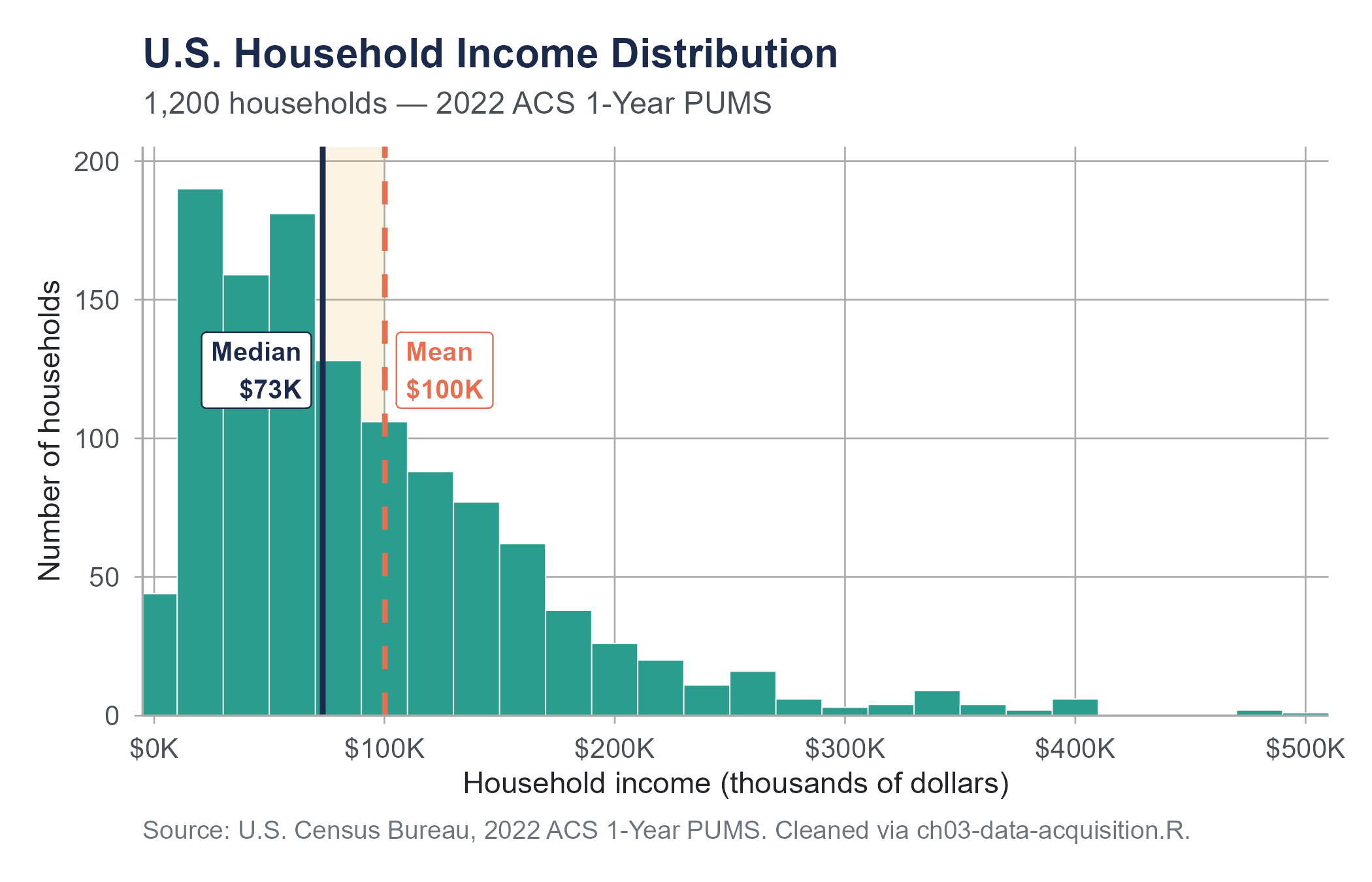
Consider household income in the United States. According to the U.S. Census Bureau, the median household income in 2022 was approximately $74,580. The mean household income, calculated by the same bureau using the same data, was considerably higher, around $105,000. That is a gap of roughly $30,000 between two numbers that both claim to represent the “typical” American household.

The gap exists because income in the United States is heavily right-skewed. Most households earn somewhere between $30,000 and $100,000. But a relatively small number of households earn far more — hundreds of thousands, millions, or even billions per year. Those extreme values pull the mean upward while barely affecting the median. A politician who wants to paint a rosy picture reports the mean. A politician who wants to highlight the struggles of working families reports the median. Both are “correct.” Neither is complete.

Figure 3.1: U.S. household income distribution with the mean and median marked. The right-skewed shape pulls the mean well above the median, illustrating how the choice of summary statistic can tell very different stories about the same data. Source: U.S. Census Bureau, 2022 ACS 1-Year PUMS.

This chapter is about the numbers we use to summarize data, what they tell us, what they hide, and how to choose among them wisely. By the end of it, you will understand why that $30,000 gap exists, why it matters, and how to avoid being fooled by someone else’s choice of summary statistic.

3.2 Measures of Center

When someone asks, “What is the typical value in this dataset?”, they are asking for a measure of center. There are three common answers to that question, and they do not always agree.

3.2.1 The Mean

The mean is the arithmetic average. Add up all the values, divide by how many there are. If you have five test scores of 72, 85, 90, 68, and 95, the mean is

\[\bar{x} = \frac{72 + 85 + 90 + 68 + 95}{5} = \frac{410}{5} = 82\]

More formally, for a dataset with $n$ observations $x_1, x_2, \ldots, x_n$, the sample mean is

\[\bar{x} = \frac{1}{n}\sum_{i=1}^{n} x_i\]

The mean is the most widely used measure of center. It has nice mathematical properties, it uses every value in the dataset, and it forms the basis of many statistical procedures we will encounter later in this book.

But the mean has a weakness. It is sensitive to extreme values. Suppose one of those five students missed most of the semester and scored a 15 instead of a 95. The mean drops from 82 to 66, even though four of the five scores are unchanged. A single extreme value pulled the center of the data in its direction.

This sensitivity is exactly what creates the gap between mean and median household income. Bill Gates walks into a diner with nine other people. Before he arrived, the mean net worth of the people in the room was maybe $50,000. Now it is over ten billion dollars. Nothing about the financial reality of those nine people changed, but the mean tells a very different story.

3.2.2 The Median

The median is the middle value when the data is arranged in order. Half the observations fall below it, half fall above it.

To find the median, sort the data from smallest to largest. If the number of observations is odd, the median is the middle value. If the number of observations is even, the median is the average of the two middle values.

For the original five test scores, sorted: 68, 72, 85, 90, 95. The median is 85, the value in position 3.

Now replace 95 with 15: 15, 68, 72, 85, 90. The median is 72. It changed, but not nearly as dramatically as the mean did. The median is resistant to extreme values, meaning that outliers do not pull it around the way they pull the mean.

This resistance is why economists and government agencies typically report median household income rather than mean household income when they want to describe what life is like for a typical family. The median says, “Half of households earn less than this, and half earn more.” It is not distorted by the fortunes of billionaires.

3.2.3 The Mode

The mode is the most frequently occurring value in a dataset. In the set 3, 5, 5, 7, 8, the mode is 5. In the set 2, 2, 4, 4, 6, there are two modes (2 and 4), making the distribution bimodal. Some datasets have no repeated values at all, in which case the mode is not particularly useful.

The mode is the only measure of center that works for categorical data. If you survey 200 people about their favorite season and 78 say autumn, 52 say summer, 41 say spring, and 29 say winter, the mode is autumn. You cannot calculate a mean or median for seasons.

For numerical data, the mode is less commonly reported than the mean or median. But it becomes useful when you want to describe the shape of a distribution, particularly when that distribution has more than one peak.

3.2.4 When to Use Which

The choice between mean, median, and mode is not arbitrary. It depends on the data.

Use the mean when the data is roughly symmetric and has no extreme outliers. The mean uses all the information in the dataset and is the foundation of many inferential methods. For symmetric distributions, the mean and median will be close to each other anyway.

Use the median when the data is skewed or contains outliers. Income, home prices, hospital bills, commute times, and many other real-world variables are right-skewed, with a long tail of high values. For these, the median better represents what a typical observation looks like.

Use the mode for categorical data or when you specifically want to identify the most common category or value. The mode can also be informative for numerical data when the distribution is bimodal, revealing that the data may contain two distinct groups.

Here is a practical guideline. If you compute both the mean and the median and they are close together, the data is probably roughly symmetric and either measure works well. If they are far apart, the data is skewed, and you should think carefully about which one answers the question you are actually asking.

The choice matters in everyday life more than most people realize. Consider a housing market scenario that plays out in cities across the country. Imagine a real estate website reporting that the “average home price” in a particular suburb is $620,000. Prospective buyers visit the neighborhood expecting to find homes near that price point, but most of the houses are priced between $280,000 and $400,000. The average is inflated by a handful of newly built luxury properties on large lots, including one listed at $4.2 million. The median home price, around $345,000, would have painted a far more accurate picture of what a typical buyer could expect to find. This pattern, a small number of high-end properties pulling the mean well above what most buyers will encounter, is characteristic of any market with substantial price variation at the top.

This is not an unusual scenario. It plays out in every city where a few high-end properties coexist with a larger stock of modest homes. Real estate agents know this, and the savvier ones choose their statistics deliberately. An agent trying to attract wealthy buyers to a neighborhood will quote the mean. An agent trying to reassure a young couple that a neighborhood is affordable will quote the median. Both are telling the truth. Both are also being strategic about which truth to tell.

The same dynamic appears in salary negotiations. A company might report that the “average salary” for its employees is $95,000. That sounds impressive until you learn that the median is $62,000, and the average is pulled up by a few executives earning seven figures. A job candidate who walks into an interview expecting $95,000 based on the average may be disappointed. The median would have set more realistic expectations.

Note

The relationship between mean and median can tell you the direction of skewness. In a right-skewed distribution (long tail to the right), the mean is greater than the median, because the extreme high values pull the mean upward. In a left-skewed distribution (long tail to the left), the mean is less than the median. This is not a perfect diagnostic, but it is a useful rule of thumb. The income data is a textbook case. Mean income exceeds median income in virtually every country on Earth, because income distributions are almost universally right-skewed.

3.3 Why Measures of Center Are Not Enough

Imagine two classes of 20 students each take the same exam. Both classes have a mean score of 75. Are these two classes performing similarly?

Not necessarily. In Class A, every student scored between 70 and 80. In Class B, half the students scored around 95 and the other half scored around 55. The averages are identical, but the student experiences are completely different. Class A is consistent. Class B is split.

The mean told you where the center is. It told you nothing about how spread out the data is around that center. For that, you need measures of spread, also called measures of variability or dispersion.

This is more than an academic point. It has life-or-death consequences in fields like medicine. Consider two hospitals that both report an average surgical wait time of 14 days. At Hospital A, every patient waits between 12 and 16 days. The process is predictable, and patients can plan around it. At Hospital B, some patients are seen within 2 days while others wait 45 days. The average is the same, but the patient experience could hardly be more different. A patient at Hospital B faces real uncertainty about when they will receive care, and those stuck in the long tail of the wait time distribution may suffer worsening conditions. Reporting only the average conceals a serious problem in the way care is distributed.

Try It Online

The Datasaurus Explorer shows a set of datasets that all share the same mean, standard deviation, and correlation, yet look completely different when plotted. Open it now, before reading further. The visual makes the chapter’s argument more forcefully than any example in text can.

The same principle applies in manufacturing. A pharmaceutical company producing pills with a target dosage of 200 milligrams needs to care about more than the average dosage across a batch. If the average is 200 mg but individual pills range from 150 mg to 250 mg, patients are receiving inconsistent and potentially dangerous doses. The spread of the data, beyond its center, determines whether the product is safe.

Measures of spread answer the question, “How much do the values in this dataset differ from one another?” A small spread means the values are clustered tightly around the center. A large spread means they are scattered widely.

3.4 Measures of Spread

3.4.1 The Range

The simplest measure of spread is the range, which is the difference between the maximum and minimum values.

\[\text{Range} = \text{Maximum} - \text{Minimum}\]

For the test scores 68, 72, 85, 90, 95, the range is $95 - 68 = 27$.

The range is easy to compute and easy to understand. But it has a serious limitation: it depends on only two values, the largest and the smallest. One extreme observation can dramatically inflate the range, and the range tells you nothing about how the rest of the data is distributed between those two extremes.

Consider two datasets. Dataset A contains the values 50, 51, 52, 53, 54, 55, 100. Dataset B contains 50, 60, 70, 80, 90, 95, 100. Both have a range of 50, but they look very different. In Dataset A, most values are clustered around 50, with a single outlier at 100. In Dataset B, the values are spread evenly across the range. The range cannot distinguish between these situations.

3.4.2 The Interquartile Range (IQR)

A more resistant measure of spread is the interquartile range, or IQR. Rather than looking at the full range from minimum to maximum, the IQR measures the range of the middle 50% of the data.

\[\text{IQR} = Q_3 - Q_1\]

where $Q_1$ is the first quartile (25th percentile) and $Q_3$ is the third quartile (75th percentile). We will define quartiles more precisely in a moment, but the idea is straightforward. $Q_1$ is the value below which 25% of the data falls, and $Q_3$ is the value below which 75% of the data falls. The IQR tells you how wide the middle half of the distribution is.

Because the IQR ignores the most extreme values at both ends, it is resistant to outliers, just as the median is resistant to outliers as a measure of center. The IQR is the natural companion to the median, and the two are often reported together.

3.4.3 Variance and Standard Deviation

The range and IQR tell you about the spread of data using just a few selected values. The variance and standard deviation take a different approach. They measure how far, on average, each observation is from the mean. These are the most commonly used measures of spread in statistical practice, and they are worth understanding in detail.

Let us build the intuition step by step.

Step 1: Deviations from the mean. For each observation, calculate how far it is from the mean. If the mean is $\bar{x}$ and an observation is $x_i$, the deviation is $x_i - \bar{x}$. Some deviations will be positive (values above the mean) and some will be negative (values below the mean).

Consider a small dataset: 4, 7, 8, 11, 15. The mean is $\bar{x} = \frac{4 + 7 + 8 + 11 + 15}{5} = 9$. The deviations are:

Observation ($x_i$)	Deviation ($x_i - \bar{x}$)
4	$4 - 9 = -5$
7	$7 - 9 = -2$
8	$8 - 9 = -1$
11	$11 - 9 = 2$
15	$15 - 9 = 6$

Step 2: Why not just average the deviations? You might think we could measure spread by averaging these deviations. The problem is that the positive and negative deviations always cancel out. Try it: $(-5) + (-2) + (-1) + 2 + 6 = 0$. The sum of the deviations from the mean is always zero. This is a mathematical property of the mean, not a coincidence.

Step 3: Squaring the deviations. To prevent the cancellation, we square each deviation. Squaring makes every value positive, and it gives extra weight to large deviations, which is often desirable because large deviations represent observations that are far from the center.

Observation ($x_i$)	Deviation ($x_i - \bar{x}$)	Squared Deviation $(x_i - \bar{x})^2$
4	$-5$	25
7	$-2$	4
8	$-1$	1
11	2	4
15	6	36

Step 4: Computing the sample variance. Sum the squared deviations and divide, but not by $n$. For a sample, we divide by $n - 1$ rather than $n$, so the result is not a simple average. The reason involves a concept called degrees of freedom, which we will address more thoroughly in later chapters. The short version is that a sample mean was used to compute the deviations, and using the sample mean rather than the true population mean uses up one degree of freedom. Dividing by $n - 1$ corrects for the fact that a sample tends to underestimate the true variability of the population.

The sample variance is

\[s^2 = \frac{1}{n-1}\sum_{i=1}^{n}(x_i - \bar{x})^2\]

For our example:

\[s^2 = \frac{25 + 4 + 1 + 4 + 36}{5 - 1} = \frac{70}{4} = 17.5\]

Step 5: Taking the square root. The variance is in squared units. If your data is measured in dollars, the variance is in “squared dollars,” which is not a meaningful quantity. Taking the square root of the variance returns us to the original units and gives us the sample standard deviation.

\[s = \sqrt{s^2} = \sqrt{17.5} \approx 4.18\]

The standard deviation tells you, roughly, how far a typical observation is from the mean. For this dataset, observations are, on average, about 4.18 units away from the mean of 9.

Note

You might wonder why we bother with variance at all, given that the standard deviation is more interpretable. The reason is that variance has cleaner mathematical properties. When you combine independent random variables, their variances add. Standard deviations do not. This property becomes essential in probability theory and inferential statistics, which is why variance appears in nearly every formula from Chapter 5 onward. Think of variance as the quantity that makes the math work and standard deviation as the quantity that makes the interpretation work.

3.4.4 Population vs. Sample Notation

Throughout this book, we distinguish between a population parameter and a sample statistic. The population mean is denoted $\mu$ (the Greek letter mu), and the population standard deviation is denoted $\sigma$ (sigma). When we calculate these from sample data, we use $\bar{x}$ for the mean and $s$ for the standard deviation.

The population variance formula divides by $N$ (the population size):

\[\sigma^2 = \frac{1}{N}\sum_{i=1}^{N}(x_i - \mu)^2\]

The sample variance formula divides by $n - 1$:

\[s^2 = \frac{1}{n-1}\sum_{i=1}^{n}(x_i - \bar{x})^2\]

In practice, you will almost always be working with samples, so the $n - 1$ version is the one to use unless you are told explicitly that your data represents the entire population.

3.4.5 Interpreting the Standard Deviation

The standard deviation is a central summary number in statistics, and developing an intuition for it will serve you well. Here are some guidelines for interpretation.

A standard deviation of zero means there is no spread at all. Every observation is the same.

A small standard deviation relative to the mean indicates that observations are tightly clustered around the center. If the mean exam score is 80 and the standard deviation is 3, most students scored close to 80.

A large standard deviation relative to the mean indicates wide dispersion. If the mean exam score is 80 and the standard deviation is 20, students’ scores are scattered from very low to very high.

Here is a way to build practical intuition for the standard deviation. Think of it as a “typical distance from the center.” When a weather forecaster says that the average high temperature in July in Phoenix is 106 degrees Fahrenheit with a standard deviation of about 4 degrees, you know that most July days will be within a few degrees of 106. A day of 114 degrees would be two standard deviations above the mean, which is unusual but not unprecedented. A day of 90 degrees would be four standard deviations below the mean, which would be so unusual it would make the news. The standard deviation gives you a ruler for measuring how surprising any particular value is. Once you develop this habit of thinking, “How many standard deviations away is that?”, you will find yourself applying it everywhere, from stock market returns to your morning commute to the number of points your favorite basketball team scores per game.

The coefficient of variation provides a way to compare spread across datasets with different scales. It is the standard deviation divided by the mean, often expressed as a percentage:

\[CV = \frac{s}{\bar{x}} \times 100\%\]

If one factory produces bolts with a mean length of 10 cm and a standard deviation of 0.5 cm, and another produces beams with a mean length of 500 cm and a standard deviation of 2 cm, which process is more variable? The bolt factory has a CV of 5%, while the beam factory has a CV of 0.4%. Relative to what it is producing, the bolt factory has more variability.

3.5 Percentiles, Quartiles, and the Five-Number Summary

3.5.1 Percentiles

A percentile tells you the value below which a given percentage of the data falls. If your score on a standardized test is at the 85th percentile, that means 85% of test-takers scored below you. The percentile is not a percentage score on the test itself. You could score 72% of the questions correctly and still be at the 85th percentile if most people scored below 72%.

More formally, the $p$th percentile is the value such that $p$% of the observations fall at or below it.

Percentiles are used constantly in practical settings. Pediatricians track children’s height and weight by percentile. Standardized tests report percentile ranks. Economic researchers use percentiles to describe income distributions with more nuance than a single number allows.

3.5.2 Quartiles

Quartiles divide the data into four equal parts using three specific percentiles.

$Q_1$ (first quartile) = 25th percentile. One quarter of the data falls below this value.
$Q_2$ (second quartile) = 50th percentile = the median. Half the data falls below this value.
$Q_3$ (third quartile) = 75th percentile. Three quarters of the data falls below this value.

To compute quartiles by hand, first sort the data and find the median. Then find the median of the lower half of the data (that gives you $Q_1$) and the median of the upper half (that gives you $Q_3$).

Consider the sorted dataset: 12, 15, 18, 22, 25, 28, 30, 33, 40.

There are 9 values. The median ($Q_2$) is the 5th value, which is 25.

The lower half is 12, 15, 18, 22. The median of this group is $\frac{15 + 18}{2} = 16.5$, so $Q_1 = 16.5$.

The upper half is 28, 30, 33, 40. The median of this group is $\frac{30 + 33}{2} = 31.5$, so $Q_3 = 31.5$.

The IQR is $Q_3 - Q_1 = 31.5 - 16.5 = 15$.

Note that different software packages use slightly different algorithms to compute quartiles, so you may occasionally see small differences depending on which tool you use. Even within R, the base quantile() function offers nine different definitions, and this can cause confusion when students compare their homework answers. The differences are typically small, often just a fraction of a unit, and they vanish entirely for large datasets. The conceptual interpretation is the same regardless of the method, so do not lose sleep over which algorithm your software uses. The important thing is understanding what the quartiles represent, not matching numbers to the last decimal place.

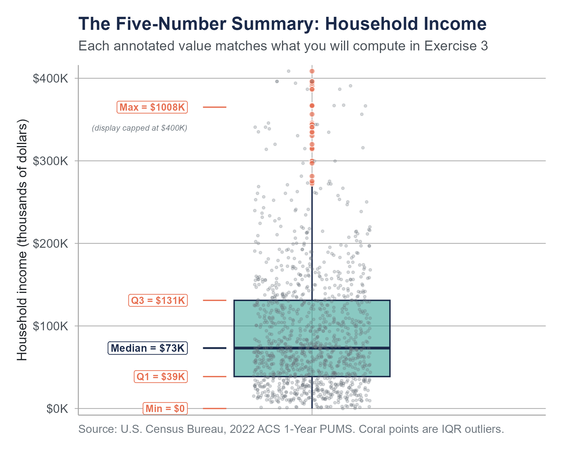
3.5.3 The Five-Number Summary

The five-number summary consists of five values that provide a compact description of a dataset’s distribution.

Minimum (the smallest value)
$Q_1$ (the first quartile)
Median (the second quartile)
$Q_3$ (the third quartile)
Maximum (the largest value)

For the dataset above, the five-number summary is: 12, 16.5, 25, 31.5, 40.

These five numbers tell you a lot. The minimum and maximum give you the range. $Q_1$ and $Q_3$ give you the IQR. The median gives you the center. The spacing between consecutive values tells you about the shape. If the distance from $Q_1$ to the median is much smaller than the distance from the median to $Q_3$, the upper half of the distribution is more spread out than the lower half, suggesting right skewness.

Figure 3.2: A box plot of U.S. household income data with all five summary statistics annotated, alongside jittered data points showing the underlying distribution. The box plot compresses the entire distribution into a compact display built from the minimum, Q1, median, Q3, and maximum. Source: U.S. Census Bureau, 2022 ACS 1-Year PUMS.

The five-number summary is the foundation of the box plot, a visual display we will explore in Chapter 4. For now, just know that box plots are graphical representations of the five-number summary, with extensions for identifying potential outliers.

3.5.4 Describing the Income Distribution with Percentiles

Returning to U.S. household income, percentiles give us a much richer picture than any single number can. Data from the Economic Policy Institute and the U.S. Census Bureau allow us to see the full distribution.

In 2022, the approximate percentile breakdown for annual household income looked something like this:

Percentile	Approximate Income
10th	$16,800
25th ($Q_1$)	$33,000
50th (Median)	$74,580
75th ($Q_3$)	$133,000
90th	$213,000
95th	$295,000
99th	$600,000+

Source: U.S. Census Bureau, Current Population Survey Annual Social and Economic Supplement, 2022; Economic Policy Institute State of Working America Data Library. These figures represent the national household income distribution and are not drawn from the acs-household-income.csv exercise dataset, which contains approximately 1,200 sampled households.

Look at the spacing. The distance from the 10th percentile to the median is about $57,780. The distance from the median to the 90th percentile is about $138,420. The upper half of the income distribution is far more spread out than the lower half. And the gap from the 90th to the 99th percentile, roughly $387,000, is wider than the entire range from the 10th to the 90th. This is what extreme right skewness looks like in a real dataset. It is also why the gap between mean and median income is so large.

The IQR for household income is approximately $133,000 $-$ $33,000 = $100,000. This tells you that the middle 50% of American households earn between roughly $33,000 and $133,000 per year. That is itself a wide range, reflecting substantial economic diversity even within the middle half of the distribution.

3.6 Outliers

3.6.1 What Is an Outlier?

An outlier is an observation that is unusually far from the rest of the data. There is no universal agreement on exactly how far “unusually far” means, but there are standard methods for detecting them.

The word “outlier” sounds technical, but the concept is intuitive. If you are looking at the salaries of employees in a small company and most earn between $40,000 and $90,000, a salary of $2,500,000 would be an outlier. It does not fit the general pattern.

Outliers can arise for several reasons, and understanding why an outlier exists is more important than deciding what to do with it mechanically.

Data entry errors. Someone typed 5000 instead of 50. This is a mistake, and fixing or removing it is straightforward and appropriate.

Measurement errors. A scale was miscalibrated. A sensor malfunctioned. Again, these errors should be corrected if possible.

Extreme but legitimate observations. Some values are far from the rest and belong there. Jeff Bezos’s income is an outlier in any sample of American incomes, but it is not an error. It is a real value that reflects something meaningful about the economy.

Different populations. An outlier may indicate that the observation comes from a different group than the rest of the data. If you are measuring the weights of house cats and one “cat” weighs 400 pounds, you may have accidentally included a lion.

The history of science is full of cases where outliers turned out to be the most interesting part of the data. In the 1990s, astronomers studying distant supernovae noticed that some of their brightness measurements did not fit the expected pattern. Rather than discarding these outliers, they investigated further and discovered that the expansion of the universe was accelerating, a finding that upended cosmology and earned the 2011 Nobel Prize in Physics. On the other hand, history is full of cases where outliers were simply measurement errors. In September 2011, physicists at the OPERA experiment reported that neutrinos traveling from CERN in Switzerland to a detector in Gran Sasso, Italy appeared to arrive about 60 nanoseconds faster than light, a result that would have overturned a century of physics. Rather than immediately announcing a discovery, the team spent months checking their equipment. In February 2012, they identified two sources of systematic error: a loose fiber optic cable connector and an oscillator running at the wrong frequency. Both issues had introduced a consistent bias into the timing measurements. The anomalous results were not a breakthrough. They were a hardware problem masquerading as a signal. The lesson the OPERA team drew, and that the scientific community drew from the episode, is exactly the right one: when a measurement is far from what theory and prior evidence predict, the first hypothesis is usually instrument or process error, not a new law of nature.

The lesson is that outliers demand attention, not automatic deletion. They are signals that something unusual is happening, and the analyst’s job is to figure out whether that something is a discovery, an error, or simply a reflection of natural variation in a messy world.

3.6.2 Detecting Outliers with the IQR Method

The most common method for identifying potential outliers uses the IQR. It defines boundaries called fences beyond which observations are flagged as potential outliers.

Lower fence = $Q_1 - 1.5 \times \text{IQR}$

Upper fence = $Q_3 + 1.5 \times \text{IQR}$

Any observation below the lower fence or above the upper fence is considered a potential outlier.

Let us work through an example. Suppose you have the following dataset of monthly electric bills (in dollars) for 15 households:

45, 52, 58, 62, 65, 68, 70, 72, 75, 80, 85, 92, 98, 110, 310

First, find the quartiles. There are 15 observations.

The median is the 8th value: 72.

The lower half is 45, 52, 58, 62, 65, 68, 70. The median of this group (the 4th value) is 62. So $Q_1 = 62$.

The upper half is 75, 80, 85, 92, 98, 110, 310. The median of this group is 92. So $Q_3 = 92$.

$\text{IQR} = 92 - 62 = 30$

Lower fence: $62 - 1.5(30) = 62 - 45 = 17$

Upper fence: $92 + 1.5(30) = 92 + 45 = 137$

No values fall below 17, so there are no low outliers. The value 310 exceeds 137, so it is flagged as a potential outlier.

The word “potential” matters. The IQR method identifies observations that are unusually far from the bulk of the data. It does not tell you whether those observations are errors, interesting phenomena, or something else entirely. That determination requires judgment and context.

3.6.3 The Ethics of Outlier Removal

Deciding what to do with outliers is one of the most consequential choices a data analyst makes, and one of the most ethically fraught.

Ethics Moment

Removing outliers changes your results. Sometimes dramatically. An analyst studying CEO compensation who removes the top 1% of earners will report a very different picture than one who keeps them in. A pharmaceutical researcher who drops patients with extreme side effects will present a rosier picture of drug safety than one who includes them. A school district that excludes the lowest-performing students from its average test scores will look more successful than it actually is.

None of these removals are inherently wrong. Outlier removal can be justified when values are clearly erroneous or when they come from a different population than the one you intend to study. But removal must be transparent. If you remove outliers, you should report that you did so, explain why, and show what the results look like both with and without the removed observations.

The danger is not in removing outliers. The danger is in removing them selectively, keeping the ones that support your conclusion and discarding the ones that do not, without telling anyone. This practice, whether intentional or unconscious, is a form of data manipulation. It can make a failing drug look effective, a bad policy look successful, or an unequal economy look fair. The rule is simple: if you would be embarrassed to explain your outlier removal decision to a skeptical colleague, you probably should not be making it.

AI Reality Check

When asked to “clean” a dataset, AI tools often flag and remove outliers mechanically, applying rules like “drop anything beyond 1.5 times the IQR” without asking whether those values are errors or legitimate observations. A large language model asked to prepare income data for analysis might automatically remove a household earning $310,000 because it exceeds the upper fence, destroying the very signal you are trying to study. The tool treats outlier detection as a cleaning step rather than an investigation step.

AI tools also tend to default to the mean when asked for “the average,” even when the data is heavily skewed and the median would be far more appropriate. Ask an AI to summarize a dataset of home prices in a neighborhood with one mansion, and it will likely report a mean that no typical home comes close to. It will do this confidently, without flagging that the distribution is skewed or that the median tells a more honest story.

The chapter’s lesson applies directly here: outliers demand investigation, not automatic deletion, and the choice between mean and median requires understanding the shape of your data. These are judgment calls that no algorithm should make for you.

3.6.4 How Outliers Affect Summary Statistics

The practical impact of outliers on summary statistics is worth seeing with concrete numbers.

Consider the following dataset of 10 home prices (in thousands of dollars) in a neighborhood:

185, 192, 205, 210, 218, 225, 230, 240, 255, 1850

Without the outlier (1850), the mean is about $217,800 and the median is $218,000. With the outlier included, the mean jumps to about $381,000 while the median changes only to $221,500. The standard deviation goes from about $22,500 to about $516,600.

A real estate agent who reports the mean home price as $381,000 is technically correct but seriously misleading. Nine of the ten homes sold for under $260,000. The median tells the true story of what a typical buyer should expect to pay.

This example illustrates why resistant statistics (summary statistics that are not strongly affected by outliers or extreme values) are often preferable when outliers are present or suspected. The median and IQR are the two most common resistant statistics. They are not immune to outliers, but they are far less affected by them than the mean and standard deviation.

3.7 Putting It All Together

Let us apply everything from this chapter to a single dataset to see how these measures work in concert.

The Economic Policy Institute publishes data on average hourly wages by income percentile in the United States. Suppose we have the following simplified dataset of annual incomes (in thousands of dollars) for 20 workers sampled from a mid-sized American city:

22, 28, 31, 34, 36, 38, 40, 42, 44, 47, 50, 53, 56, 60, 65, 72, 85, 105, 140, 310

In the exercises that follow, you will apply these same methods to a much larger dataset of 1,200 households drawn from the 2022 American Community Survey. The concepts are identical; only the scale changes.

Mean:

\[\bar{x} = \frac{22 + 28 + 31 + \cdots + 140 + 310}{20} = \frac{1,358}{20} = 67.9\]

The mean income in this sample is $67,900.

Median:

With 20 values, the median is the average of the 10th and 11th values. The sorted data is already in order, so the median is $\frac{47 + 50}{2} = 48.5$, or $48,500.

The mean is about $19,400 higher than the median. This tells us the data is right-skewed, pulled upward by the high earners.

Quartiles and IQR:

$Q_1$ is the median of the lower 10 values (22, 28, 31, 34, 36, 38, 40, 42, 44, 47). With 10 values, $Q_1 = \frac{36 + 38}{2} = 37$, or $37,000.

$Q_3$ is the median of the upper 10 values (50, 53, 56, 60, 65, 72, 85, 105, 140, 310). $Q_3 = \frac{65 + 72}{2} = 68.5$, or $68,500.

$\text{IQR} = 68.5 - 37 = 31.5$, or $31,500.

Five-Number Summary:

Minimum = 22, $Q_1$ = 37, Median = 48.5, $Q_3$ = 68.5, Maximum = 310.

(All in thousands of dollars.)

Outlier Detection:

Lower fence: $37 - 1.5(31.5) = 37 - 47.25 = -10.25$

Upper fence: $68.5 + 1.5(31.5) = 68.5 + 47.25 = 115.75$

No values fall below the lower fence. Two values, 140 and 310, exceed the upper fence of 115.75 and are flagged as potential outliers.

Standard Deviation:

Computing this by hand for 20 values is tedious, but working through the formula:

\[s = \sqrt{\frac{1}{19}\sum_{i=1}^{20}(x_i - 67.9)^2}\, \approx 56.9\]

The standard deviation is about $56,900. This is large relative to the mean, confirming that the data has substantial spread. The coefficient of variation is $\frac{56.9}{67.9} \times 100\% \approx 83.8\%$, which is high, indicating substantial variability in incomes.

What the numbers tell us together. The mean ($67,900) substantially exceeds the median ($48,500), confirming right skewness. The IQR ($31,500) is much smaller than the range ($288,000), indicating that the range is heavily influenced by extreme values. The two flagged outliers at $140,000 and $310,000 are driving much of the discrepancy between the mean and the median. If a reporter wanted to describe the typical income in this sample, the median would be the better choice. If a researcher wanted to describe the total economic output of the group, the mean (or the sum) would be more relevant.

This is the key lesson. No single summary statistic is always right or always wrong. The right statistic depends on the question you are asking.

It is worth noting that this kind of analysis is far from an academic exercise. Journalists, policy analysts, and researchers make these choices every day. When the Bureau of Labor Statistics releases its monthly jobs report, the numbers that make headlines are themselves summary statistics chosen from a much larger set of available data. The unemployment rate is a kind of proportion. The number of jobs added is a count. The average hourly wage is a mean. Each tells a different story about the labor market, and each can be used selectively to support a particular narrative. A reader who understands the material in this chapter is better equipped to ask the right follow-up questions. When someone tells you “the average is X,” you should wonder about the median. When someone tells you a group is performing well “on average,” you should ask about the spread. These are not pedantic questions. They are the difference between understanding the data and being misled by it.

3.8 A Note on Income Data

The income data used throughout this chapter comes primarily from two sources. The U.S. Census Bureau’s Current Population Survey and American Community Survey are among the primary official sources for household income data in the United States. These surveys sample tens of thousands of households annually and produce the official income statistics cited by government agencies, researchers, and the media.

The Economic Policy Institute (EPI) publishes detailed analyses of income and wage data, often broken down by percentile, race, gender, education level, and other categories. Their State of Working America Data Library is freely available online and provides the kind of granular data that reveals patterns invisible in national averages.

The dataset used in this chapter’s exercises (acs-household-income.csv) draws directly from the 2022 ACS 1-Year Public Use Microdata Sample. It contains approximately 1,200 households sampled to represent variation across all 50 states, five regions, and five education levels. The data acquisition and sampling script (ch03-data-acquisition.R) is available on the companion website. See Appendix B for a full description of the dataset’s variables, sampling strategy, and education level classifications.

When you encounter income data in the news or in research, two questions worth asking are, “Is this mean or median?” and “What population does this represent?” National averages can mask enormous regional and demographic variation. The median household income in San Francisco is very different from the median household income in rural Mississippi, and neither is well-represented by the national figure.

3.9 Choosing the Right Summary Statistics

The following table provides a quick reference for when to use each measure.

Situation	Measure of Center	Measure of Spread
Symmetric data, no outliers	Mean	Standard deviation
Skewed data or outliers present	Median	IQR
Categorical data	Mode	Not applicable (use frequency tables)
Comparing variability across different scales	Mean with CV	Coefficient of variation
Quick overview of distribution	Median	Five-number summary

When in doubt, report both the mean and the median. If they are close, the distribution is roughly symmetric and either works well. If they differ substantially, the discrepancy itself is informative, and you should investigate why.

3.10 Looking Ahead

Chapter 3 has given you a numerical vocabulary for describing data: where the center is, how spread out the values are, and how to identify observations that fall unusually far from the rest. Chapter 4 takes these same ideas and turns them into pictures. The five-number summary you computed here is the direct foundation of the box plot. The distinction between symmetric and skewed distributions, which we described in words here, becomes immediately visible in a histogram or density plot. The outlier-detection logic from this chapter reappears in visualizations that mark flagged observations as individual points. Numerical summaries and visual displays are not alternatives. They answer different questions about the same distribution, and the most complete analysis uses both.

3.11 Key Terms

Mean: The arithmetic average of a dataset. Calculated by summing all values and dividing by the number of observations. Notation: $\bar{x}$ for a sample mean, $\mu$ for a population mean.
Median: The middle value of a sorted dataset. Half the observations fall below it, half above.
Mode: The most frequently occurring value in a dataset. The only measure of center applicable to categorical data.
Range: The difference between the maximum and minimum values in a dataset.
Interquartile Range (IQR): The difference between the third quartile and the first quartile ($Q_3 - Q_1$). Measures the spread of the middle 50% of the data. Resistant to outliers.
Variance: The average of the squared deviations from the mean. Notation: $s^2$ for a sample, $\sigma^2$ for a population. Measured in squared units.
Standard Deviation: The square root of the variance. Measures how far, on average, observations are from the mean. Notation: $s$ for a sample, $\sigma$ for a population. Measured in the same units as the data.
Coefficient of Variation (CV): The standard deviation divided by the mean, expressed as a percentage. Useful for comparing variability across datasets with different units or scales.
Percentile: The value below which a given percentage of observations fall. The 85th percentile is the value below which 85% of observations fall.
Quartiles: The 25th ($Q_1$), 50th ($Q_2$, also the median), and 75th ($Q_3$) percentiles. They divide the sorted data into four equal parts.
Five-Number Summary: A set of five descriptive statistics consisting of the minimum, $Q_1$, median, $Q_3$, and maximum. Provides a compact overview of the distribution.
Outlier: An observation that is unusually far from the rest of the data. Often identified using the IQR method (values beyond $Q_1 - 1.5 \times \text{IQR}$ or $Q_3 + 1.5 \times \text{IQR}$).
Fences: The boundaries used in the IQR method for identifying potential outliers. The lower fence is $Q_1 - 1.5 \times \text{IQR}$ and the upper fence is $Q_3 + 1.5 \times \text{IQR}$. Observations beyond the fences are flagged as potential outliers.
Resistant Statistic: A summary statistic that is not strongly affected by outliers or extreme values. The median and IQR are resistant. The mean and standard deviation are not.
Skewness: A measure of the asymmetry of a distribution. Right-skewed distributions have a long tail to the right (mean > median). Left-skewed distributions have a long tail to the left (mean < median).
Bimodal: A distribution with two distinct peaks, suggesting the data may contain two subgroups.
Degrees of Freedom: The number of independent pieces of information in the data. In the context of sample variance, this is $n - 1$, reflecting the constraint that the deviations from the sample mean must sum to zero. The concept reappears in later chapters with the t, chi-square, and F distributions.

3.12 Further Reading and References

The following works are cited in this chapter or provide valuable additional context.

On U.S. household income data: U.S. Census Bureau. (2023). Income in the United States: 2022 (Current Population Reports, P60-279). U.S. Government Publishing Office. The primary source for official household income statistics, including the $74,580 median figure cited throughout this chapter.

Economic Policy Institute. State of Working America Data Library. Available at epi.org/data. Provides detailed percentile-level income breakdowns used in the chapter’s income distribution table.

On the chapter dataset: The income distribution discussed in this chapter is drawn directly from the 2022 ACS 1-Year Public Use Microdata Sample. The data acquisition script (ch03-data-acquisition.R) is available on the companion website.

On the OPERA neutrino episode: The OPERA Collaboration. (2012). Measurement of the neutrino velocity with the OPERA detector in the CNGS beam. Journal of High Energy Physics, 2012(10), 93. The published version contains the corrected result, consistent with the speed of light. The original anomalous claim appeared in a September 2011 preprint (arXiv:1109.4897v1). The error, traced to a loose fiber optic cable, was identified and announced by the collaboration in February 2012.

On outlier judgment in scientific practice: Baggerly, K.A., & Coombes, K.R. (2009). Deriving chemosensitivity from cell lines: Forensic bioinformatics and reproducible research in high-throughput biology. Annals of Applied Statistics, 3(4), 1309–1334. A forensic investigation into published cancer genomics results that shows what happens when outliers and data errors go uninvestigated.

For further reading on summary statistics and economic inequality: Piketty, T. (2014). Capital in the twenty-first century. Harvard University Press. (Uses income and wealth percentile data extensively; the chapter’s discussion of the gap between mean and median income connects directly to its empirical framework.)

3.13 Exercises

3.13.1 Check Your Understanding

A news headline reads, “Average American household earns over $105,000 per year.” Another headline reads, “Typical American household earns about $75,000 per year.” Both are based on the same government data. Explain how both can be correct. Which number is the mean and which is the median? Which better represents the experience of a typical household, and why?
For the dataset 3, 5, 7, 7, 8, 10, 12, calculate the mean, median, and mode. Are any of these values the same? What does this suggest about the shape of the distribution?
Explain in your own words why the sum of the deviations from the mean always equals zero. Why does this mathematical property create a problem if we want to measure how spread out the data is?
A dataset has a mean of 50 and a standard deviation of 0. What can you conclude about the values in this dataset? Explain.
Two datasets each have a mean of 100. Dataset A has a standard deviation of 5 and Dataset B has a standard deviation of 25. Describe in words what the distributions of these two datasets would look like compared to each other.
What is the difference between the range and the interquartile range? Under what circumstances would the range be a misleading measure of spread? Give a specific example.
Explain why the median is described as “resistant” to outliers while the mean is not. Illustrate your answer with a simple numerical example.
A dataset has $Q_1 = 20$, median $= 35$, and $Q_3 = 42$. Without seeing the full dataset, what can you say about the shape of the distribution? Is it symmetric, left-skewed, or right-skewed? Explain your reasoning.
The formula for sample variance divides by $n - 1$ rather than $n$. What is this adjustment called, and why is it used? You do not need to prove it mathematically, just explain the intuition.
A student calculates the mean of a dataset and gets 60. They then calculate the median and get 82. What does this tell them about the shape of the distribution? Would they expect the data to be right-skewed or left-skewed? Explain.

3.13.2 Apply It

(See Appendix B for complete variable descriptions for all datasets used in these exercises.)

For the following problems, use the acs-household-income.csv dataset available on the companion website. This dataset is drawn from the 2022 American Community Survey 1-Year Public Use Microdata Sample, produced by the U.S. Census Bureau. It contains approximately 1,200 household records representing all 50 states, sampled to reflect the national distribution of income and educational attainment. The variables are household_id (a unique identifier), state (the household’s state of residence), region (geographic region: Northeast, Southeast, Midwest, Southwest, or West), household_income (annual household income in 2022 dollars), education_level (the highest education level attained by the head of household: High School or Less, Some College or Associate, Bachelor, Master or Professional, or Doctorate), and household_size (number of people in the household).

Load the dataset and examine its structure. How many observations are there? How many variables? Identify each variable’s type (categorical or numerical). For the numerical variables, briefly describe what each one measures.
Compute the mean and median of household_income across all households. Are these two values close to each other or far apart? What does the relationship between them tell you about the shape of the income distribution in this sample? How do your sample estimates compare to the 2022 national figures cited in this chapter ($74,580 median, $105,000 mean)?
Compute the five-number summary for household_income. Report the minimum, $Q_1$, median, $Q_3$, and maximum. Calculate the IQR. Interpret these values in the context of household income inequality.
Group the data by state. For each state, compute the mean and median household_income. Identify the five states with the highest mean household income. For each of these states, compute the difference between the mean and the median. Which state has the largest gap? What does a larger gap suggest about the income distribution within that state?
Using the IQR method on the full household_income variable, check whether any individual households are outliers. Show your fence calculations. How many households are flagged as outliers? Are the outliers concentrated in any particular states or regions?
Group the data by education_level. For each group, compute the mean, standard deviation, and coefficient of variation of household_income. Which education level has the most variability in absolute terms (largest SD)? Which has the most variability in relative terms (largest CV)? Does the Some College or Associate group behave as you would expect given its position between High School or Less and Bachelor? What does this tell you about income variation across education levels?
Choose any single state that has at least 10 households in the dataset. For that state, compute the 10th, 25th, 50th, 75th, and 90th percentiles of household_income. Compute the approximate range (P90 - P10) and the IQR (P75 - P25). What fraction of the approximate range is captured by the IQR? How does this compare to what you would expect for a symmetric distribution?
Group the data by region. For each region, compute the mean, median, and standard deviation of household_income. Which region has the highest mean? Which has the largest standard deviation? Do the mean and median differ substantially within any region, suggesting skewness?
Create a new variable called the “income gap ratio” for each state, defined as the ratio of the 90th percentile of household_income to the 10th percentile of household_income within that state (use only states with at least 10 observations). Compute this ratio for all qualifying states. What is the mean and median of this ratio across states? Which state has the highest ratio, and which has the lowest? What does this ratio capture about within-state inequality?
Pick three states: one with a high median income, one near the overall sample median, and one with a low median income. For each, compute the five-number summary of household_income. Compare the three distributions. Where do you see the largest differences, at the bottom, the middle, or the top of the income distribution?
Pick any 10 households from the dataset. Compute their sample variance and sample standard deviation by hand using the formulas $s^2 = \frac{1}{n-1}\sum(x_i - \bar{x})^2$ and $s = \sqrt{s^2}$. Show each step: the mean, each $(x_i - \bar{x})$, each squared deviation, the sum, the division by $n - 1$, and the square root. Then verify your answer with R’s var() and sd(). Why does the formula divide by $n - 1$ rather than $n$? Tie your answer back to the conceptual question in Check Your Understanding problem 9.

3.13.3 Think Deeper

Politicians sometimes argue about whether the economy is “working” by citing different summary statistics. One camp cites GDP growth and mean incomes, pointing to expansion. The other cites median wages and cost-of-living data, pointing to stagnation for ordinary families. Is one side “right” and the other “wrong”? Or are they answering different questions? What set of summary statistics would you recommend for an honest, comprehensive assessment of economic well-being? Justify your choices.
A hospital administrator reports that the average emergency room wait time is 45 minutes. Patient advocacy groups counter that most patients wait over an hour. Explain how both claims could be true simultaneously. What additional information would you want before deciding which statistic better represents the patient experience? Discuss the ethical responsibility of the hospital when choosing which number to report publicly.
An analyst studying housing affordability removes all homes priced above $2 million from the dataset before computing average home prices, arguing that luxury homes are “not relevant” to the typical buyer. Is this a defensible decision? Under what circumstances would it be appropriate, and under what circumstances would it be misleading? How should the analyst communicate this decision in a published report?
Consider two school districts. District A has a mean math score of 78 with a standard deviation of 5. District B has a mean math score of 78 with a standard deviation of 18. The districts serve similar demographics. Which district is performing better, and why? A parent asks, “Is my child more likely to get a good education in District A or District B?” How would you answer this question using the concepts from this chapter? What additional information would you want?
The Gini coefficient condenses an entire income distribution into a single number between 0 and 1. What information is lost in this compression? Two countries could have the same Gini coefficient but very different income distributions. Construct a hypothetical example of two such countries and explain how summarizing complex data with a single number can obscure important differences. When, if ever, is a single summary statistic sufficient for making a policy decision?

Observation (\(x_i\))	Deviation (\(x_i - \bar{x}\))
4	\(4 - 9 = -5\)
7	\(7 - 9 = -2\)
8	\(8 - 9 = -1\)
11	\(11 - 9 = 2\)
15	\(15 - 9 = 6\)

Observation (\(x_i\))	Deviation (\(x_i - \bar{x}\))	Squared Deviation \((x_i - \bar{x})^2\)
4	\(-5\)	25
7	\(-2\)	4
8	\(-1\)	1
11	2	4
15	6	36