9 Comparing Groups
9.1 Are Emily and Greg More Employable Than Lakisha and Jamal?
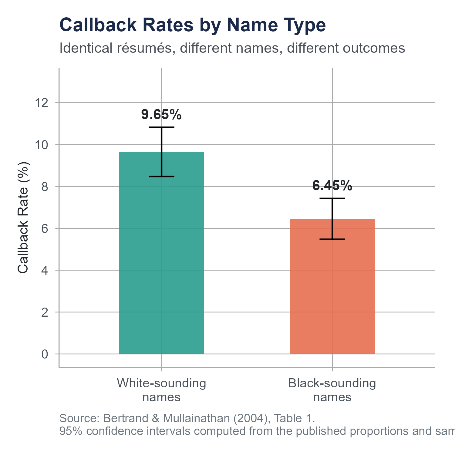
In 2004, economists Marianne Bertrand and Sendhil Mullainathan published an experiment that was as simple in design as it was sobering in its findings. They created roughly 5,000 fictitious résumés and sent them in response to help-wanted ads in Boston and Chicago newspapers. The résumés were carefully constructed to be equivalent in quality, some with stronger credentials and some with weaker ones, but otherwise matched on experience, education, and formatting. The only thing the researchers varied was the name at the top.
Half the résumés were assigned names that, based on prior surveys, were strongly associated with being White. Names like Emily Walsh, Greg Baker, Brendan Murray, Anne Ryan. The other half were assigned names strongly associated with being Black. Names like Lakisha Washington, Jamal Jones, Tamika Williams, Aisha Harris. (The last names here are illustrative; the original study used first names only as the experimental treatment.) Everything else about the paired résumés was identical or statistically equivalent.
Then the researchers waited for the phone to ring.
Résumés with White-sounding names received a callback about once in every 10 sent. Résumés with Black-sounding names received a callback about once in every 15. That is roughly a 50% gap in callback rates, driven entirely by the name at the top of the page, which served as a proxy for perceived race. The gap was consistent across occupations, industries, and employer sizes.
Here is what made the finding even more troubling. When the researchers improved the quality of the résumés by adding more experience, better credentials, and stronger formatting, the callback rate for White-sounding names jumped noticeably. For Black-sounding names, higher quality résumés produced almost no additional benefit. The labor market was rewarding credentials for one group and largely ignoring them for another.
The paper has been widely cited in labor economics. It is also, at its core, a study about comparing groups. Two groups of résumés, identical except for the name, sent into the same labor market, and the outcome measured across both groups. The statistical question is straightforward. Is the difference in callback rates between these two groups large enough that we can rule out random chance as the explanation?
That is the kind of question this chapter teaches you to answer. But we are going to go beyond two groups. What happens when you have three groups, or five, or ten? What changes in your analysis when you move from comparing two means to comparing many? And what responsibilities come with analyzing group differences, especially when those differences involve race, gender, disability, income, or any other dimension along which people have been historically sorted and ranked?
This chapter marks the beginning of Part III of this book. In Parts I and II, you built the foundations: how to summarize data, how to think about probability, how to construct confidence intervals, and how to test hypotheses. Now we start applying those tools to increasingly realistic questions. Comparing groups is where statistics meets the messiness of the social world, where the numbers carry both uncertainty and meaning, and where the analyst’s choices about framing and interpretation carry real consequences for real people.
9.2 The Problem with Running Multiple t-Tests
In Chapter 8, you learned to use a two-sample t-test to compare the means of two groups. If you want to know whether the average callback rate differs between résumés with White-sounding names and résumés with Black-sounding names, a two-sample t-test handles that cleanly. Two groups, one comparison, one test.
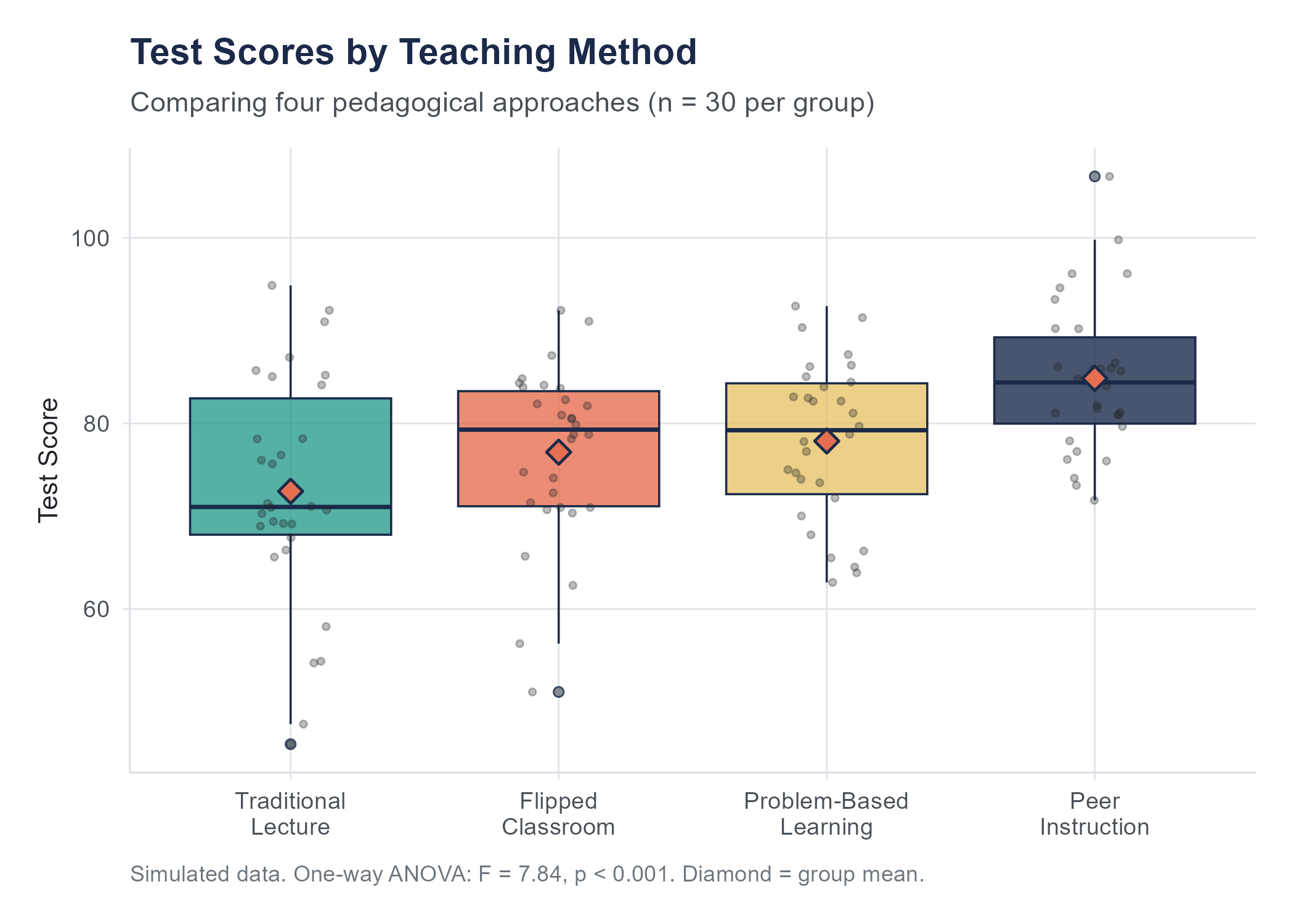
But suppose your research question is more complex. Imagine you are studying the effectiveness of four different teaching methods on exam scores. You have Group A (traditional lecture), Group B (flipped classroom), Group C (problem-based learning), and Group D (peer instruction). You want to know whether any of these methods produce different average exam scores.
Your first instinct might be to run all possible pairwise t-tests. Compare A to B. Compare A to C. Compare A to D. Compare B to C. Compare B to D. Compare C to D. That is six comparisons. With four groups, the number of pairwise comparisons is \(\binom{4}{2} = 6\). With five groups it would be 10. With ten groups, 45.
This seems thorough. It is actually dangerous.
Here is the problem. Each t-test you run at the \(\alpha = 0.05\) significance level has a 5% chance of producing a false positive, a Type I error, even when there is no real difference between the groups. If you run one test, your chance of at least one false positive is 5%. If you run six independent tests, each at 5%, the probability of getting at least one false positive is no longer 5%. It is
\[P(\text{at least one Type I error}) = 1 - (1 - \alpha)^k\]
where \(k\) is the number of comparisons. For six tests at \(\alpha = 0.05\), this gives
\[1 - (1 - 0.05)^6 = 1 - (0.95)^6 = 1 - 0.7351 = 0.2649\]
That is roughly a 26% chance of at least one false positive. You started with a 5% threshold because you wanted to be reasonably sure your findings were not due to chance. By running six tests, you have inflated your actual error rate to more than one in four. Run 20 comparisons and your probability of at least one false positive exceeds 64%. You are now more likely than not to “find” a difference that does not exist.
This is the multiple comparisons problem, sometimes called the problem of multiplicity. It is not a minor technical nuisance. It is a common way that researchers fool themselves and their audiences. Every additional comparison you run is another lottery ticket for a false positive. Buy enough tickets and you will eventually “win.”
The multiple comparisons problem shows up far beyond formal hypothesis testing. Data journalists sometimes compare crime rates across dozens of cities and highlight whichever comparison looks most dramatic. Marketing analysts test ten different email subject lines and declare a winner after each line was tested on a small subsample. In each case, the more comparisons you make, the more likely you are to find something that looks like a pattern but is just noise. The first question to ask when someone presents a surprising group difference is always, “How many comparisons did they run to find this one?”
9.3 ANOVA: The Big Picture
Analysis of Variance, universally abbreviated as ANOVA, solves the multiple comparisons problem by testing all the groups at once. Instead of asking “Is Group A different from Group B?” and “Is Group A different from Group C?” and so on, ANOVA asks a single omnibus question.
“Is there any difference among the group means, or are they all essentially the same?”
More precisely, the null and alternative hypotheses for a one-way ANOVA are
\[H_0: \mu_1 = \mu_2 = \mu_3 = \cdots = \mu_k\]
\[H_A: \text{At least one } \mu_i \text{ differs from the others}\]
where \(\mu_1, \mu_2, \ldots, \mu_k\) are the population means of the \(k\) groups. The null hypothesis says all the groups have the same population mean. The alternative says at least one group’s mean is different from at least one other group’s mean. It does not say which groups differ or how many differ. Just that the means are not all equal.
This single test controls the Type I error rate at \(\alpha\) across all groups simultaneously. You run one test, you get one p-value, and that p-value reflects the overall evidence against the null hypothesis that all group means are equal. No inflation. No lottery tickets.
The name “Analysis of Variance” is admittedly confusing when you first encounter it, because the method is used to compare means, not variances. But the name makes sense once you understand the logic, which is that ANOVA compares means by analyzing variances. Specifically, it compares two types of variability.
9.4 The F-Statistic: Between vs. Within
The core idea of ANOVA is surprisingly intuitive. Imagine you are looking at data from three groups. Each group has some spread in its values, and the group means are at different locations. The question ANOVA asks is this: are the group means more spread out than you would expect given how much variability exists within each group?
Think of it this way. Suppose three classes of students take the same exam. Class 1 averages 74, Class 2 averages 76, and Class 3 averages 75. The means are slightly different, but within each class the scores range from about 50 to 95. The means barely budge compared to the wide spread of individual scores within each class. That small wiggle among the means could easily be due to the random mix of students in each class. ANOVA would probably not reject the null hypothesis.
Now suppose the three class averages are 62, 78, and 91, while within each class the scores only range from about 5 points below the mean to 5 points above. The means are spread far apart relative to how tightly packed the individual scores are within each class. It would be very hard to explain that pattern by random variation alone. ANOVA would almost certainly reject the null hypothesis.
This is the logic of the F-statistic. It is a ratio.
\[F = \frac{\text{variability between groups}}{\text{variability within groups}}\]
When the group means are far apart relative to the spread within each group, the F-statistic is large. When the group means are close together relative to the within-group spread, the F-statistic is small, close to 1. An F-statistic of 1 means the between-group variability is about the same as the within-group variability, exactly what you would expect if the groups all came from the same population.
Here is another way to think about it. Imagine you are standing in a hallway and you can hear three different conversations happening in three rooms. If the rooms are full of people who are all talking at roughly the same volume (lots of within-group noise) and the three conversations are about equally loud on average (little between-group difference), you would have a hard time telling the rooms apart from the hallway. But if one room is whispering, one is speaking normally, and one is practically shouting, and within each room people are fairly consistent, you would immediately notice that the rooms are different. ANOVA formalizes that intuition. The question is always whether the signal between groups rises above the noise within groups.
9.4.1 Making It Precise
Let us formalize this. Suppose you have \(k\) groups, with \(n_i\) observations in group \(i\) and a total of \(N = n_1 + n_2 + \cdots + n_k\) observations overall. Let \(\bar{x}_i\) be the mean of group \(i\) and \(\bar{x}\) be the overall mean of all observations combined, often called the grand mean.
The total variability in the data can be decomposed into two pieces.
Between-group variability measures how much the group means differ from the grand mean.
\[SS_{\text{between}} = \sum_{i=1}^{k} n_i (\bar{x}_i - \bar{x})^2\]
Each group mean’s distance from the grand mean is squared, weighted by the group size, and summed up. If the group means are all equal to the grand mean, this quantity is zero. The more the group means spread out, the larger it gets.
Within-group variability measures how much individual observations differ from their own group mean.
\[SS_{\text{within}} = \sum_{i=1}^{k} \sum_{j=1}^{n_i} (x_{ij} - \bar{x}_i)^2\]
This is the pooled variability inside all the groups. It captures the “noise” or natural spread that exists even within a single group. Think of it as the variability that has nothing to do with group membership.
The total sum of squares is
\[SS_{\text{total}} = SS_{\text{between}} + SS_{\text{within}}\]
This decomposition is fundamental. The total variability in your data can be split into the part explained by group membership and the part that remains unexplained, just the natural scatter within groups.
To compute the F-statistic, we need to convert these sums of squares into mean squares by dividing by their respective degrees of freedom.
\[MS_{\text{between}} = \frac{SS_{\text{between}}}{k - 1}\]
\[MS_{\text{within}} = \frac{SS_{\text{within}}}{N - k}\]
The between-group degrees of freedom are \(k - 1\) because \(k\) group means have \(k - 1\) independent pieces of information after accounting for the grand mean. The within-group degrees of freedom are \(N - k\) because \(N\) total observations lose \(k\) degrees of freedom from estimating the \(k\) group means.
The F-statistic is then
\[F = \frac{MS_{\text{between}}}{MS_{\text{within}}}\]
This statistic follows an F-distribution with \(k - 1\) and \(N - k\) degrees of freedom, assuming the null hypothesis is true. The F-distribution is always positive and right-skewed. Under the null hypothesis, the expected value of \(F\) is approximately 1. Values much larger than 1 provide evidence against the null hypothesis.
9.4.2 The ANOVA Table
Results from an ANOVA are traditionally presented in a table that organizes all of these pieces.
| Source | Sum of Squares | df | Mean Square | F | p-value |
|---|---|---|---|---|---|
| Between groups | \(SS_{\text{between}}\) | \(k - 1\) | \(MS_{\text{between}}\) | \(F\) | \(p\) |
| Within groups | \(SS_{\text{within}}\) | \(N - k\) | \(MS_{\text{within}}\) | ||
| Total | \(SS_{\text{total}}\) | \(N - 1\) |
You will see this table in virtually every piece of statistical software. Learning to read it is essential.
9.4.3 A Worked Example
A researcher wants to know whether background music affects concentration. The researcher recruits 30 participants and randomly assigns 10 to each of three conditions: silence, classical music, and pop music with lyrics. Each participant completes a timed concentration task, and the researcher records the number of errors. The data produce the following group statistics.
| Group | \(n\) | Mean errors | Standard deviation |
|---|---|---|---|
| Silence | 10 | 4.2 | 1.8 |
| Classical | 10 | 5.1 | 2.0 |
| Pop with lyrics | 10 | 7.8 | 2.3 |
The grand mean is \(\bar{x} = \frac{10(4.2) + 10(5.1) + 10(7.8)}{30} = \frac{171}{30} = 5.7\).
Between-group sum of squares.
\[SS_{\text{between}} = 10(4.2 - 5.7)^2 + 10(5.1 - 5.7)^2 + 10(7.8 - 5.7)^2\]
\[= 10(2.25) + 10(0.36) + 10(4.41) = 22.5 + 3.6 + 44.1 = 70.2\]
Within-group sum of squares. Using the relationship \(SS_{\text{within}} = \sum_{i=1}^{k}(n_i - 1)s_i^2\), we get
\[\begin{aligned} SS_{\text{within}} &= 9(1.8)^2 + 9(2.0)^2 + 9(2.3)^2 \\ &= 9(3.24) + 9(4.00) + 9(5.29) \\ &= 29.16 + 36.00 + 47.61 = 112.77 \end{aligned}\]
Mean squares.
\[MS_{\text{between}} = \frac{70.2}{3 - 1} = \frac{70.2}{2} = 35.1\]
\[MS_{\text{within}} = \frac{112.77}{30 - 3} = \frac{112.77}{27} = 4.177\]
F-statistic.
\[F = \frac{35.1}{4.177} = 8.40\]
With \(df_1 = 2\) and \(df_2 = 27\), an F-statistic of 8.40 yields a p-value of approximately 0.0015. At the \(\alpha = 0.05\) level, we reject the null hypothesis and conclude that the mean number of errors is not the same across all three music conditions.
But here is a critical point. The F-test tells us that the three group means are not all equal. It does not tell us which groups differ from which. Is silence different from pop? Is classical different from pop? Is silence different from classical? The omnibus F-test cannot answer these questions. For that, we need post-hoc tests.
9.5 Assumptions of ANOVA
Before we move to post-hoc comparisons, let us be clear about what ANOVA requires to be trustworthy. There are three main assumptions, and they parallel the assumptions you encountered with t-tests.
9.5.1 Independence
The observations must be independent of one another. One participant’s score should not influence another participant’s score. Random assignment to groups (in an experiment) or random sampling from populations (in an observational study) generally ensures independence. Violations of independence are serious and can badly distort both the F-statistic and the p-value.
Common violations include repeated measures on the same participants (for which you need repeated-measures ANOVA, a topic for a more advanced course), clustering (students nested within classrooms, patients nested within hospitals), and time-series data where observations close in time are correlated.
9.5.2 Normality
ANOVA assumes that the observations within each group come from normally distributed populations. In practice, this assumption is less fragile than it sounds. The F-test is moderately resistant to violations of normality, especially when sample sizes are reasonably large and roughly equal across groups. A common rule of thumb is that with about 20 or more observations per group the Central Limit Theorem provides enough cover for the F-test even when individual observations are not normal. This is a heuristic, not a hard cutoff, and one you will see across most introductory and applied statistics texts.
With small samples and heavily skewed data, the normality assumption becomes more important. You can check it by examining histograms or normal probability plots of the data within each group. If the data look severely non-normal and your groups are small, you might consider a nonparametric alternative like the Kruskal-Wallis test (introduced in Chapter 8 alongside the Wilcoxon tests), which works on the ranks of the data and does not assume normality.
9.5.3 Equal Variances (Homogeneity of Variance)
ANOVA assumes that the population variances are the same across all groups. This is sometimes called the homogeneity of variance or homoscedasticity assumption. You can check it informally by comparing the standard deviations across groups. A common rule of thumb is that ANOVA is reasonably trustworthy as long as the largest group standard deviation is no more than about twice the smallest group standard deviation.
For a more formal check, Levene’s test evaluates whether the group variances are statistically distinguishable. If you find evidence of unequal variances, you can use Welch’s ANOVA, which adjusts the degrees of freedom to account for the heterogeneity, much as Welch’s t-test does for the two-group case.
In our music and concentration example, the standard deviations were 1.8, 2.0, and 2.3. The ratio of the largest to the smallest is \(2.3 / 1.8 = 1.28\), well within the rule-of-thumb guideline. The equal variance assumption looks reasonable here.
9.6 Post-Hoc Tests: Finding Where the Differences Are
You have run your ANOVA and obtained a small p-value. You can conclude that the group means are not all equal. Now what?
You want to know which specific groups differ from which. This is the job of post-hoc tests (from the Latin for “after this”). These are pairwise comparisons that are run only after a statistically meaningful F-test, and they include adjustments to control the overall Type I error rate.
9.6.1 Tukey’s Honestly Significant Difference (HSD)
The most widely used post-hoc test is Tukey’s HSD, developed by the statistician John Tukey. It compares every possible pair of group means while controlling the family-wise error rate at \(\alpha\).
For each pair of groups \(i\) and \(j\), the Tukey HSD computes
\[q = \frac{\bar{x}_i - \bar{x}_j}{\sqrt{MS_{\text{within}} / n}}\]
where \(n\) is the number of observations per group (assuming equal group sizes) and \(q\) is compared to the studentized range distribution with parameters \(k\) (the number of groups) and \(N - k\) (the within-group degrees of freedom).
In the case of unequal group sizes, a modified version called the Tukey-Kramer method is used, replacing \(n\) with a harmonic mean or adjusting the standard error for each pair. Most statistical software handles this automatically.
Tukey’s HSD produces a confidence interval and a p-value for each pairwise comparison. A pair of groups is considered different if the confidence interval for their mean difference does not include zero, or equivalently, if the adjusted p-value is less than \(\alpha\).
Returning to our music and concentration example, Tukey’s HSD would compare three pairs.
| Comparison | Difference in means | Adjusted p-value | Conclusion |
|---|---|---|---|
| Silence vs. Classical | \(5.1 - 4.2 = 0.9\) | 0.578 | Not distinguishable |
| Silence vs. Pop | \(7.8 - 4.2 = 3.6\) | 0.001 | Different |
| Classical vs. Pop | \(7.8 - 5.1 = 2.7\) | 0.014 | Different |
The pattern is clear. Pop music with lyrics leads to more errors than either silence or classical music. Silence and classical music do not produce distinguishably different error counts. The overall F-test told us something was different. Tukey’s HSD told us what.
9.6.2 Other Post-Hoc Options
Tukey’s HSD is not the only post-hoc procedure. Others you may encounter include
Bonferroni correction. Divide your significance level \(\alpha\) by the number of comparisons. With three comparisons at \(\alpha = 0.05\), each comparison is tested at \(0.05 / 3 = 0.0167\). This is simple and conservative, meaning it is less likely to find differences that are real but also less likely to produce false positives. The Bonferroni correction works with any type of test, not just ANOVA follow-ups.
Scheffé’s method. The most conservative of the common post-hoc tests. It controls the Type I error rate for all possible contrasts, not just pairwise comparisons. Because it is so conservative, it has less power to detect real differences.
Dunnett’s test. Used when you want to compare each group to a single control group, rather than comparing all groups to each other. If you have one control condition and three treatment conditions, Dunnett’s test makes only three comparisons instead of six.
For most introductory applications, Tukey’s HSD is the standard choice. It balances Type I error control with statistical power and is available in every major statistics package.
In practice, you do not compute post-hoc tests by hand. R handles the bookkeeping: TukeyHSD() follows the base aov() function and produces a table of pairwise comparisons with adjusted p-values and confidence intervals. The companion R walkthrough on this book’s website shows the full sequence end to end (fit the ANOVA, check assumptions, apply Tukey’s HSD, and report effect sizes) for the music-and-concentration example used in this section. The point of doing the calculation by hand on a small example, as we did above, is to make the logic concrete, not to suggest you would ever need to do it that way for real data.
One important detail about post-hoc tests. They should only be conducted after a statistically meaningful omnibus F-test. If the overall ANOVA fails to reject the null hypothesis, there is no justification for hunting through pairwise comparisons looking for differences. The F-test is the gatekeeper. If it says “no convincing evidence that the means differ,” you should not go looking for differences anyway, because any you find are likely to be Type I errors. Some researchers ignore this convention and run pairwise comparisons regardless, which brings you right back to the multiple comparisons problem that ANOVA was designed to avoid.
There is an exception worth mentioning. If you had planned comparisons (also called a priori contrasts) specified before collecting data, you can test those specific comparisons without first running an omnibus F-test. Planned comparisons are hypothesis-driven, not data-driven, and they carry less risk of capitalizing on chance. For example, if a researcher studying four teaching methods had a specific theory that problem-based learning would outperform traditional lecture, they could test that one comparison directly. The key is that the comparison was specified before looking at the data, not selected after seeing which means happened to be the farthest apart.
John Tukey, who developed the HSD test, was a prolific statistician of the twentieth century. He also invented the box plot, is credited with early published uses of the terms “bit” (for binary digit) and “software,” and developed the Fast Fourier Transform algorithm with James Cooley. His 1977 book Exploratory Data Analysis helped shift statistics from a purely confirmatory discipline to one that also valued looking at data with fresh eyes before testing hypotheses. If you find yourself appreciating a box plot, you have Tukey to thank.
9.7 Effect Sizes for Group Comparisons
A small p-value tells you that the group means are probably not all equal. It does not tell you how much they differ, or whether the difference matters in practical terms. For that, you need an effect size.
9.7.1 Eta-Squared (\(\eta^2\))
The most common effect size for ANOVA is eta-squared, defined as
\[\eta^2 = \frac{SS_{\text{between}}}{SS_{\text{total}}}\]
Eta-squared represents the proportion of total variability in the outcome that is accounted for by group membership. It ranges from 0 to 1. An \(\eta^2\) of 0.10 means that 10% of the variability in the outcome is associated with group differences. The remaining 90% is within-group variability.
In our music and concentration example
\[\eta^2 = \frac{70.2}{70.2 + 112.77} = \frac{70.2}{182.97} = 0.384\]
About 38% of the variability in concentration errors is accounted for by the music condition. That is a large effect by conventional standards.
Cohen’s (1988) guidelines for interpreting \(\eta^2\) are
| \(\eta^2\) | Interpretation |
|---|---|
| 0.01 | Small effect |
| 0.06 | Medium effect |
| 0.14 | Large effect |
These are rough benchmarks, not rigid rules. A “small” effect in medicine might save thousands of lives. A “large” effect in education might be driven by a poorly designed study. Always interpret effect sizes in context.
9.7.2 Partial Eta-Squared (\(\eta_p^2\))
When your ANOVA includes more than one factor (for example, music condition and time of day), partial eta-squared becomes the preferred measure. It represents the proportion of variance accounted for by a particular factor, after removing the variance accounted for by other factors.
\[\eta_p^2 = \frac{SS_{\text{effect}}}{SS_{\text{effect}} + SS_{\text{error}}}\]
In a one-way ANOVA with a single factor, partial eta-squared and eta-squared are identical. The distinction only matters when you have multiple factors, which is the setting of factorial ANOVA, typically covered in a second statistics course. For now, just know that partial eta-squared exists and is what most software reports by default in multi-factor designs.
9.7.3 Cramér’s V for Categorical Comparisons
Eta-squared applies when your outcome variable is numerical and you are comparing means. But what if both your grouping variable and your outcome are categorical? The Bertrand and Mullainathan study is a good example. The grouping variable is the name type (White-sounding vs. Black-sounding), and the outcome is whether the resume received a callback (yes or no). Both are categorical. Here you would use a chi-square test (as you learned in Chapter 8), and the appropriate effect size is Cramér’s V.
Cramér’s V is defined as
\[V = \sqrt{\frac{\chi^2}{n \times (m - 1)}}\]
where \(\chi^2\) is the chi-square test statistic, \(n\) is the total sample size, and \(m\) is the smaller of the number of rows or the number of columns in the contingency table.
Cramér’s V ranges from 0 to 1. A value of 0 means no association between the variables. A value of 1 means a perfect association. For a 2-by-2 table, Cramér’s V is identical to the absolute value of the phi coefficient (\(\phi\)).
Guidelines for interpreting Cramér’s V depend on the size of the table. For a 2-by-2 table
| Cramér’s V | Interpretation |
|---|---|
| 0.10 | Small association |
| 0.30 | Medium association |
| 0.50 | Large association |
For larger tables, the thresholds are lower because the degrees of freedom increase.
9.8 When to Use Which Test: A Decision Framework
At this point, you have encountered several tests for comparing groups. Here is a framework to help you choose the right one.
Step 1: What type is your outcome variable?
If your outcome is numerical (continuous or discrete quantities like test scores, incomes, wait times), you reach for t-tests or ANOVA.
If your outcome is categorical (counts or proportions, like callback vs. no callback, party affiliation, disease status), you reach for chi-square tests.
Step 2: How many groups are you comparing?
If you are comparing exactly two groups on a numerical outcome, use a two-sample t-test (or its Welch variant if variances are unequal).
If you are comparing three or more groups on a numerical outcome, use a one-way ANOVA, followed by post-hoc tests if the F-test is statistically meaningful.
If you are comparing the distribution of a categorical outcome across two or more groups, use a chi-square test of independence (or Fisher’s exact test if expected cell counts are very small).
Step 3: Are your groups independent or related?
If the groups contain different individuals (as in a between-subjects experiment or comparing different populations), use the independent-samples versions of these tests.
If the groups contain the same individuals measured at different times or under different conditions, you need the paired or repeated-measures versions (paired t-test, repeated-measures ANOVA). These are not the focus of this chapter but are important to recognize.
Here is the framework in table form.
| Outcome type | Number of groups | Groups independent? | Test |
|---|---|---|---|
| Numerical | 2 | Yes | Two-sample t-test |
| Numerical | 2 | No (paired) | Paired t-test |
| Numerical | 3 or more | Yes | One-way ANOVA |
| Numerical | 3 or more | No (repeated) | Repeated-measures ANOVA |
| Categorical | 2 or more | Yes | Chi-square test of independence |
This table covers the most common scenarios. Real research sometimes calls for more specialized methods, but if you can navigate this decision tree, you can handle the vast majority of group comparison problems.
A few additional considerations when choosing your test.
Sample size matters. With very small samples (fewer than 5 per group), the assumptions of ANOVA and the chi-square test become harder to justify. For small-sample ANOVA with non-normal data, the Kruskal-Wallis test (Chapter 8) is the rank-based alternative. For chi-square tests with small expected cell counts (typically less than 5), Fisher’s exact test is the recommended substitute. Fisher’s exact test computes the p-value directly from the hypergeometric distribution rather than relying on the chi-square approximation, which is why it remains valid in small-sample situations where the chi-square approximation would not be. R’s fisher.test() produces it in one line.
Ordinal outcomes fall in a gray area. If your outcome is ordinal, like a satisfaction rating on a 1-to-5 scale, you have a choice. Many researchers treat ordinal data as numerical and use ANOVA, especially when the scale has five or more levels and the data are reasonably symmetric. Others prefer nonparametric methods like the Kruskal-Wallis test, which makes fewer assumptions about the measurement scale. There is no universal consensus. The choice depends on the specific data, the number of scale points, and how comfortable you are treating the distances between levels as approximately equal.
The relationship between the t-test and ANOVA. When you have exactly two groups, a one-way ANOVA and a two-sample t-test give identical results. The F-statistic equals the square of the t-statistic (\(F = t^2\)), and the p-values are the same. ANOVA generalizes the t-test to more than two groups. If someone asks you whether to use a t-test or ANOVA for two groups, the honest answer is that it does not matter, you will get the same answer either way.
9.9 Beyond the Résumé Study: ANOVA in Practice
Let us work through a more extended example to see how all these pieces fit together in practice.
A public health researcher wants to know whether awareness of nutrition labeling differs across four regions of the United States (Northeast, Southeast, Midwest, and West). The researcher surveys a random sample of adults from each region and administers a nutrition knowledge quiz scored from 0 to 100. The results produce the following data.
| Region | \(n\) | Mean score | Standard deviation |
|---|---|---|---|
| Northeast | 45 | 68.3 | 12.1 |
| Southeast | 52 | 61.7 | 14.5 |
| Midwest | 48 | 64.9 | 11.8 |
| West | 50 | 70.2 | 13.0 |
Total \(N = 195\). Number of groups \(k = 4\).
Step 1: Check assumptions.
Independence. The participants were randomly sampled from each region independently. This assumption appears met.
Normality. With group sizes ranging from 45 to 52, the Central Limit Theorem provides adequate coverage even if the underlying distributions are somewhat non-normal. The researcher checks histograms and finds no severe skewness.
Equal variances. The standard deviations range from 11.8 to 14.5. The ratio of the largest to the smallest is \(14.5 / 11.8 = 1.23\), well within the guideline of 2. The equal variance assumption appears reasonable.
Step 2: Compute the grand mean.
\[\begin{aligned} \bar{x} &= \frac{45(68.3) + 52(61.7) + 48(64.9) + 50(70.2)}{195} \\ &= \frac{3073.5 + 3208.4 + 3115.2 + 3510.0}{195} = \frac{12907.1}{195} = 66.19 \end{aligned}\]
Step 3: Compute the between-group sum of squares.
\[\begin{aligned} SS_{\text{between}} &= 45(68.3 - 66.19)^2 + 52(61.7 - 66.19)^2 \\ &\quad + 48(64.9 - 66.19)^2 + 50(70.2 - 66.19)^2 \end{aligned}\]
\[= 45(4.4521) + 52(20.1601) + 48(1.6641) + 50(16.0801)\]
\[= 200.34 + 1048.33 + 79.88 + 804.01 = 2132.56\]
Step 4: Compute the within-group sum of squares.
\[SS_{\text{within}} = 44(12.1)^2 + 51(14.5)^2 + 47(11.8)^2 + 49(13.0)^2\]
\[= 44(146.41) + 51(210.25) + 47(139.24) + 49(169.00)\]
\[= 6442.04 + 10722.75 + 6544.28 + 8281.00 = 31990.07\]
Step 5: Compute mean squares and the F-statistic.
\[MS_{\text{between}} = \frac{2132.56}{4 - 1} = \frac{2132.56}{3} = 710.85\]
\[MS_{\text{within}} = \frac{31990.07}{195 - 4} = \frac{31990.07}{191} = 167.49\]
\[F = \frac{710.85}{167.49} = 4.24\]
Step 6: Find the p-value. With \(df_1 = 3\) and \(df_2 = 191\), an F-statistic of 4.24 yields a p-value of approximately 0.006.
Step 7: Interpret. At \(\alpha = 0.05\), we reject the null hypothesis. The data provide convincing evidence that mean nutrition knowledge scores differ across the four regions.
Step 8: Post-hoc comparisons. Tukey’s HSD reveals that the Southeast differs from both the Northeast (\(p = 0.042\)) and the West (\(p = 0.003\)). No other pairwise differences are statistically distinguishable at \(\alpha = 0.05\).
Step 9: Effect size.
\[\eta^2 = \frac{2132.56}{2132.56 + 31990.07} = \frac{2132.56}{34122.63} = 0.062\]
About 6% of the variability in nutrition knowledge scores is associated with region. By Cohen’s guidelines, this is a medium effect. Region plays a measurable but modest role in explaining differences in nutrition knowledge.
Notice the interplay between statistical meaning and practical meaning in this example. The p-value of 0.006 tells us we have strong evidence that the regional means are not all equal. The \(\eta^2\) of 0.062 tells us that region explains about 6% of the variation, which leaves 94% explained by other factors, things like individual education, socioeconomic status, access to healthcare, cultural food practices, and personal interest in nutrition. A statistically detectable difference is not necessarily a large or important one. The effect size helps you keep perspective.
9.10 The Ethics of Comparing Groups
Every time you compare groups, you make a choice about framing. How you describe the groups, what language you use, and what explanations you offer for any differences you find all carry ethical weight. Nowhere is this more important than when the groups are defined by race, gender, socioeconomic status, disability, or other dimensions of identity.
Deficit framing occurs when researchers describe group differences in a way that locates the problem within the group that scores lower, rather than in the systems and structures that produce the disparity.
Consider the National Assessment of Educational Progress (NAEP), sometimes called “The Nation’s Report Card.” NAEP data consistently show that Black and Hispanic students score lower on average than White students in reading and mathematics. This pattern has been described for decades as the “achievement gap.”
That term, “achievement gap,” is a deficit frame. It centers the analysis on what certain groups of students have not achieved. It subtly implies that the explanation lies within the students or their families or their cultures. It directs attention away from the systems that produced the disparity, including unequal school funding, residential segregation, differential access to experienced teachers, and the long-term consequences of discriminatory policies in housing, lending, and employment.
An alternative framing is the “opportunity gap” or the “education debt,” a term used by education scholar Gloria Ladson-Billings. This framing asks not “Why are these students scoring lower?” but “What resources, opportunities, and supports have been systematically withheld from these students?” The data are the same. The statistical analysis is the same. The interpretation shifts from blaming the group to examining the system.
The same issue arises in public health. The CDC Wonder database shows large disparities in life expectancy, infant mortality, and chronic disease prevalence across racial groups. Reporting that “Black Americans have higher rates of hypertension” is a factual statement, but without context it can slide into deficit framing. The context matters. Decades of research have linked these disparities to residential segregation, environmental racism, unequal access to healthcare, the physiological effects of chronic stress from discrimination, and the historical exclusion of Black Americans from wealth-building opportunities like homeownership and higher education.
When you analyze group comparisons, ask yourself these questions.
- Am I describing what the data show, or am I implying a cause that the data cannot support?
- Am I locating the “problem” within the group that scores lower, or am I examining the structures that produce the disparity?
- Would my framing read as fair to a careful reader who belongs to the group I am describing?
- Am I comparing groups to a “default” that I have left unexamined?
The goal is not to avoid making group comparisons. Group comparisons are essential for identifying disparities, documenting differential treatment, and holding institutions accountable. The Bertrand and Mullainathan study is a powerful example of a group comparison that surfaced evidence of disparate treatment. The goal is to make those comparisons with precision, honesty, and an awareness that your framing shapes how your audience understands the world.
9.11 Connecting ANOVA to the Résumé Study
The B&M study itself does not call for ANOVA; its outcome (callback or no callback) is categorical, so the right tool is a chi-square test or a two-proportion z-test. The chapter methods apply once we extend the design.
Imagine the same experiment run with three name categories (White-sounding, Black-sounding, and Hispanic-sounding) and the same yes/no callback outcome. A chi-square test of independence on the resulting 3×2 table would tell you whether callback rates differ across the three name types. If the omnibus p-value is small, follow up with pairwise chi-square tests on 2×2 subtables under a Bonferroni-corrected significance level to identify which pairs of name types differ.
Now suppose the outcome were the number of days until a callback, a numerical variable, rather than a yes/no. With three name-type groups, that is exactly the setup for a one-way ANOVA, followed by Tukey’s HSD to identify specific group differences. Same study, different measurement, different tool.
The choice of test always follows from the type of outcome variable and the number of groups. The research question determines the groups; the measurement determines the test.
Modern analytical tools and AI systems can slice data into hundreds or thousands of subgroups and test for differences across all of them in seconds. A machine learning pipeline might automatically compare outcomes across every combination of age group, gender, region, income bracket, and education level. With enough subgroups, some comparisons will produce small p-values purely by chance.
This is the multiple comparisons problem on steroids. A human researcher running six pairwise comparisons might recognize the need for a Bonferroni correction or Tukey’s HSD. An automated system running 500 comparisons might flag dozens of “differences” that are nothing but noise, and present them in a dashboard with the same visual weight as genuine findings.
The problem is compounded by the fact that automated systems do not understand context. An algorithm does not know that a 0.3-point difference in customer satisfaction between two regions is practically meaningless, even if it is statistically distinguishable with a large enough sample. It does not know that a disparity in loan approval rates between racial groups demands a fundamentally different kind of attention than a disparity in ice cream flavor preferences between age groups.
When you encounter AI-generated analyses that compare many subgroups, ask the following.
- How many comparisons were tested? If the report highlights 5 differences, were 5 comparisons run or 500?
- Was any correction applied for multiple testing? If not, expect a high proportion of false positives.
- Are the reported effect sizes practically meaningful, or just statistically detectable?
- Is the tool treating all group differences as equivalent, or does it distinguish between differences that matter and differences that do not?
The ability to run comparisons at scale is powerful. Without the statistical discipline to control error rates, it is also dangerous.
9.12 A Note on the Chi-Square Test
We introduced the chi-square concept in Chapter 8; here we apply it to comparing groups across categories.
While the focus of this chapter is ANOVA, the decision framework above includes the chi-square test, and you should understand how it connects. The chi-square test of independence evaluates whether two categorical variables are associated. You construct a contingency table showing the observed counts, calculate the expected counts under the assumption that the variables are independent, and compute
\[\chi^2 = \sum \frac{(O - E)^2}{E}\]
where \(O\) is the observed count in each cell and \(E\) is the expected count. The sum is taken over all cells in the table. Large values of \(\chi^2\) indicate that the observed data deviate from what would be expected if the variables were independent.
For the résumé study, the contingency table would look like this.
| Callback | No callback | Total | |
|---|---|---|---|
| White-sounding names | 235 | 2,200 | 2,435 |
| Black-sounding names | 157 | 2,278 | 2,435 |
| Total | 392 | 4,478 | 4,870 |
The expected count for each cell is \(\frac{\text{row total} \times \text{column total}}{\text{grand total}}\). The chi-square statistic tests whether the callback rates differ between the two name types. In this case, the answer is a clear yes.
The chi-square test generalizes to tables with more than two rows or columns. If you had three name types and two outcomes (callback vs. not), you would have a 3-by-2 table, and the chi-square test would tell you whether callback rates differ across the three name types simultaneously, controlling for multiple comparisons in the same way that ANOVA tests all group means at once.
The chi-square test has its own assumptions. The expected count in each cell of the contingency table should be at least 5 for the chi-square approximation to be reliable. If some expected counts are smaller than 5, you can combine categories if it makes substantive sense, or you can use Fisher’s exact test, which does not rely on the chi-square approximation. The observations must also be independent, meaning each case contributes to only one cell in the table.
One more parallel worth noting. Just as the F-test in ANOVA is an omnibus test that tells you something differs but not what, the chi-square test with more than two groups tells you that the distribution of outcomes is not the same across all groups, but it does not pinpoint which groups differ from which. For that, you need follow-up pairwise comparisons, typically chi-square tests on 2-by-2 subtables with a Bonferroni correction to the significance level. The logic is exactly the same as with ANOVA post-hoc testing. The omnibus test opens the door, and the pairwise comparisons tell you which rooms to look in.
9.13 Pulling It All Together
This chapter has covered a lot of ground. Let us step back and see the big picture.
You started with a simple problem: comparing groups. When you have two groups and a numerical outcome, a t-test does the job. When you have more than two groups, running multiple t-tests inflates your Type I error rate. ANOVA solves this by testing all groups simultaneously with a single F-test.
The F-statistic compares how much the group means differ from each other (between-group variability) to how much individual observations differ within their groups (within-group variability). A large F means the group means are spread out relative to the within-group noise, which is evidence that at least some groups are different.
If the F-test yields a small p-value, post-hoc tests like Tukey’s HSD identify which specific pairs of groups differ, while controlling the overall error rate. Effect sizes like eta-squared quantify how much of the total variability is explained by group membership, giving you a measure of practical importance beyond the binary of “statistically different or not.”
When your outcome is categorical rather than numerical, the chi-square test of independence serves a parallel role, and Cramér’s V provides the effect size.
Throughout all of this, the ethical imperative is clear. Group comparisons are tools for understanding the world, not for ranking people. The same analysis that documents discrimination can, if framed carelessly, reinforce the stereotypes that produce it. Your job as a statistical thinker is to let the data speak honestly while being honest about what the data cannot say.
The Bertrand and Mullainathan study did this effectively. It did not compare Black and White job applicants. It compared identical résumés with different names. The experimental design isolated the variable of interest, perceived race, from all confounding factors. The analysis documented a disparity. The interpretation correctly placed the source of that disparity not in the applicants but in the employers who evaluated them.
That is what good group comparison looks like.
One final thought before we move to the exercises. The methods in this chapter, ANOVA, chi-square tests, post-hoc comparisons, and effect sizes, are among the most widely used tools in applied statistics. They appear in medical research comparing treatments, in education research comparing curricula, in business analytics comparing customer segments, in public policy research comparing program outcomes. If you understand the logic of comparing group means and proportions, you understand a framework that extends to hundreds of practical applications.
But tools are only as good as the person using them. An ANOVA can tell you that three groups have different averages. It cannot tell you why. It cannot tell you what to do about it. It cannot tell you whether the groups were fairly defined, whether the measurements were valid, or whether your interpretation serves truth or merely confirms what you already believed. Those are human judgments, and they matter as much as the math.
In the next chapter, we move from comparing groups to modeling relationships between variables: the subject of regression. But regression, as you will see, rests on the same foundation as ANOVA. The idea that you can partition variability into explained and unexplained components, and use that partition to draw inferences, carries straight through from this chapter into the next. The tools grow more flexible, but the logic stays the same.
Open the ANOVA Visualizer on the companion website. Adjust group means and within-group variability and watch the F-statistic update in real time. Try making all group means identical and see what happens to \(F\). Then spread the means apart and see how quickly it climbs.
9.14 Looking Ahead
This chapter has given you tools for comparing groups: ANOVA for means, chi-square tests for proportions, post-hoc tests for identifying which groups differ, and effect sizes for quantifying how much they differ. But all of these methods treat the groups as the explanatory variable and ask whether the response variable differs across them. In the next chapter, we shift to a different kind of question. Instead of comparing discrete groups, we model the relationship between two continuous variables. If spending per student varies across states, and test scores vary across states, how do they vary together? How much does one variable change, on average, when the other changes by one unit? That is the subject of regression analysis, and it turns out to be a natural extension of the ANOVA framework. The idea that you can partition variation into explained and unexplained components carries straight through.
9.15 Further Reading and References
The following works are cited in this chapter or provide valuable additional context for the ideas covered here.
On the résumé audit study: Bertrand, M., & Mullainathan, S. (2004). Are Emily and Greg more employable than Lakisha and Jamal? A field experiment on labor market discrimination. American Economic Review, 94(4), 991–1013. (The widely cited study that provided this chapter’s opening example, demonstrating racial discrimination in callback rates using a randomized field experiment.)
On multiple comparisons and the false discovery problem: Benjamini, Y., & Hochberg, Y. (1995). Controlling the false discovery rate: A practical and powerful approach to multiple testing. Journal of the Royal Statistical Society: Series B, 57(1), 289–300. (The foundational paper introducing the false discovery rate procedure, an alternative to the Bonferroni correction that is less conservative and widely used in genomics, neuroscience, and other fields with large numbers of comparisons.)
On deficit framing in research: Tuck, E. (2009). Suspending damage: A letter to communities. Harvard Educational Review, 79(3), 409–428. (A foundational critique of “damage-centered research” that frames marginalized communities primarily in terms of their deficits, arguing for approaches that also document resilience, strength, and aspiration.)
On effect sizes and their interpretation: Cohen, J. (1988). Statistical power analysis for the behavioral sciences (2nd ed.). Lawrence Erlbaum Associates. (The classic reference for effect size measures including Cohen’s \(d\), \(\eta^2\), and the benchmarks for “small,” “medium,” and “large” effects that are widely used across disciplines.)
For further reading on comparing groups: Maxwell, S. E., Delaney, H. D., & Kelley, K. (2017). Designing experiments and analyzing data: A model comparison perspective (3rd ed.). Routledge. (A comprehensive treatment of ANOVA, factorial designs, repeated measures, and the relationship between ANOVA and regression.)
Ladson-Billings, G. (2006). From the achievement gap to the education debt: Understanding achievement in U.S. schools. Educational Researcher, 35(7), 3–12. (The paper that introduced the “education debt” framework discussed in this chapter’s Ethics Moment, arguing that framing disparities as “gaps” locates the problem in communities rather than in the systems that produced the disparity.)
9.16 Key Terms
- Analysis of Variance (ANOVA): A statistical method for testing whether the means of three or more groups are equal, using the F-statistic to compare between-group and within-group variability.
- Between-group variability (\(SS_{\text{between}}\)): The sum of squared differences between each group mean and the grand mean, weighted by group size. Measures how much the group means differ from each other.
- Bonferroni correction: A method for adjusting the significance level in multiple comparisons by dividing \(\alpha\) by the number of tests performed.
- Chi-square test of independence: A test for whether two categorical variables are associated, based on comparing observed cell counts to the counts expected under independence.
- Cramér’s V: An effect size measure for the association between two categorical variables, derived from the chi-square statistic. Ranges from 0 to 1.
- Deficit framing: Describing group differences in a way that locates the problem within the lower-performing group, rather than examining the structures and systems that produce the disparity.
- Degrees of freedom: In ANOVA, the between-group degrees of freedom are \(k - 1\) and the within-group degrees of freedom are \(N - k\), where \(k\) is the number of groups and \(N\) is the total sample size.
- Effect size: A measure of the magnitude of a difference or association, independent of sample size. Common effect sizes for group comparisons include eta-squared, partial eta-squared, and Cramér’s V.
- Eta-squared (\(\eta^2\)): The proportion of total variability in the outcome that is accounted for by group membership. Calculated as \(SS_{\text{between}} / SS_{\text{total}}\).
- F-distribution: The probability distribution of the F-statistic under the null hypothesis, characterized by two degrees-of-freedom parameters.
- F-statistic: The ratio of between-group mean square to within-group mean square. Large values provide evidence that the group means are not all equal.
- Family-wise error rate: The probability of making at least one Type I error across a set of multiple comparisons.
- Grand mean: The overall mean of all observations across all groups, denoted \(\bar{x}\).
- Homogeneity of variance (homoscedasticity): The assumption that all groups have the same population variance. Checked informally by comparing group standard deviations or formally using Levene’s test.
- Kruskal-Wallis test: A nonparametric alternative to one-way ANOVA that does not assume normality. Based on ranks rather than raw values.
- Levene’s test: A formal test for the equality of variances across groups.
- Mean square: A sum of squares divided by its degrees of freedom. Used to compute the F-statistic.
- Multiple comparisons problem: The inflation of the overall Type I error rate that occurs when multiple hypothesis tests are conducted simultaneously.
- One-way ANOVA: ANOVA with a single grouping variable (factor).
- Partial eta-squared (\(\eta_p^2\)): The proportion of variance accounted for by a factor after removing variance explained by other factors. Identical to eta-squared in one-way ANOVA.
- Post-hoc test: A pairwise comparison conducted after a statistically meaningful F-test to determine which specific groups differ. Examples include Tukey’s HSD, Bonferroni, and Scheffé’s method.
- Sum of squares: The sum of squared deviations used to measure variability. In ANOVA, the total sum of squares is partitioned into between-group and within-group components.
- Tukey’s Honestly Significant Difference (HSD): A post-hoc test that compares all pairs of group means while controlling the family-wise error rate.
- Welch’s ANOVA: A modification of standard ANOVA that does not assume equal variances across groups.
- Within-group variability (\(SS_{\text{within}}\)): The sum of squared differences between each observation and its group mean. Measures the natural spread of observations within groups.
A full R walkthrough of this chapter is online at stats.marginoferrormedia.com/walkthroughs/r-ch09.html. It reproduces the 9.65% / 6.45% callback rates with chisq.test(), fits a one-way ANOVA on experience by education with aov() and TukeyHSD(), computes eta-squared, and shows Kruskal-Wallis as the rank-based alternative.
9.17 Exercises
9.17.1 Check Your Understanding
Explain in your own words why running multiple t-tests to compare several group means inflates the Type I error rate. What happens to the probability of at least one false positive as the number of comparisons increases?
A one-way ANOVA produces an F-statistic of 1.03 with a p-value of 0.38. What does this tell you about the relationship between the between-group variability and the within-group variability? What do you conclude about the group means?
Describe the null and alternative hypotheses for a one-way ANOVA with five groups. Be precise about what the alternative hypothesis does and does not claim.
Why is the F-statistic always positive? Can it ever be less than 1? If so, what would that mean?
A researcher runs an ANOVA and obtains a p-value of 0.002. The researcher immediately concludes that every group mean is different from every other group mean. What is wrong with this conclusion?
What are the three main assumptions of one-way ANOVA? For each, explain what happens to the trustworthiness of the results when the assumption is violated, and name one way to check whether the assumption is met.
Explain the difference between \(SS_{\text{between}}\) and \(SS_{\text{within}}\) in your own words. What does each one measure, and how do they combine to form \(SS_{\text{total}}\)?
Why do we need post-hoc tests after a statistically meaningful F-test? Why not just look at the group means and conclude that the highest and lowest means are different?
A study reports \(\eta^2 = 0.03\) for the effect of teaching method on exam scores. The p-value is 0.01. Is the effect statistically detectable? Is it practically large? Explain the distinction.
When is a chi-square test of independence the appropriate choice instead of ANOVA? Give an example of a research question where you would use each test.
9.17.2 Apply It
(See Appendix B for complete variable descriptions for all datasets used in these exercises.)
The following exercises reference the resume-callbacks.csv dataset. This dataset contains real data from the field experiment by Bertrand and Mullainathan (2004), “Are Emily and Greg More Employable Than Lakisha and Jamal?”, sourced via the OpenIntro package. Each row represents one resume sent to an employer in response to help-wanted ads in Boston and Chicago. Variables include resume_id (a unique identifier), name_type (White-sounding or Black-sounding), gender (Male or Female, based on the first name assigned), resume_quality (High or Low), years_experience (a numerical variable), education (the level of education listed on the resume: Bachelor or High School), and callback (Yes if the resume received a callback, No otherwise).
Using the
resume-callbacks.csvdataset, construct a contingency table showing callback counts byname_type. Compute the callback rate for White-sounding names and for Black-sounding names. What is the difference in callback rates?Conduct a chi-square test of independence to test whether callback status is associated with
name_type. State the null and alternative hypotheses, report the chi-square statistic and p-value, and interpret the result. Calculate Cramér’s V and comment on the effect size.Construct a contingency table showing callback counts by
educationlevel. Is there evidence that callback rates differ across education levels? Conduct a chi-square test and report your findings.Now consider
years_experienceas the outcome variable. Compute the mean and standard deviation ofyears_experienceseparately for résumés that received a callback and those that did not. Conduct a two-sample t-test to determine whether the mean years of experience differs between the two callback groups. Report the test statistic, p-value, and your conclusion.Compute the mean and standard deviation of
years_experienceseparately for each combination ofname_typeandgender(i.e., four groups: White-sounding Female, White-sounding Male, Black-sounding Female, Black-sounding Male). Create a table showing these summary statistics. Based on a visual inspection, do the means appear to differ across the four groups?Conduct a one-way ANOVA to test whether the mean
years_experiencediffers across the fourname_type-by-gendergroups you created in the previous problem. Report the ANOVA table, including \(SS_{\text{between}}\), \(SS_{\text{within}}\), degrees of freedom, mean squares, the F-statistic, and the p-value.If your ANOVA in the previous problem produced a statistically meaningful result, conduct Tukey’s HSD post-hoc test. Which pairs of groups have statistically distinguishable mean years of experience? Present the results in a table. If the F-test was not statistically meaningful, explain why post-hoc tests should not be conducted.
Calculate \(\eta^2\) for the ANOVA from problem 6. What proportion of the variability in years of experience is accounted for by the four-group classification? How would you characterize this effect size using Cohen’s guidelines?
The dataset includes both
name_typeandresume_quality. Construct a 2-by-2-by-2 contingency table (or two separate 2-by-2 tables) to examine callback rates byname_typeseparately for low-quality and high-quality résumés. Does the gap in callback rates between name types appear to change depending on resume quality? What does this suggest about how perceived race interacts with qualifications in the labor market?Conduct a chi-square test of independence to test whether callback rates differ by
gender. Report your findings. Then conduct separate chi-square tests for the association betweenname_typeand callback within each gender group. Are the patterns consistent across gender groups, or does the magnitude of discrimination appear to differ?Re-run the four-group ANOVA on
years_experiencefrom problem 6, but this time use Welch’s ANOVA (which does not assume equal variances across groups). In R,oneway.test(years_experience ~ name_gender, data = ..., var.equal = FALSE)produces it. Compare the resulting F-statistic and p-value to your earlier classical ANOVA result. Then compute the standard deviation ofyears_experiencewithin each of the four groups. Are the variances close enough that the equal-variance assumption seems reasonable, or does the Welch correction change the conclusion in a substantive way?
9.17.3 Think Deeper
The Bertrand and Mullainathan study used names as a proxy for perceived race. Some critics argued that the names might signal socioeconomic status rather than race, and that employers might be responding to perceived social class rather than perceived race. How does this critique relate to the concept of confounding? Does it invalidate the finding that identical résumés receive different treatment based on the name? How would you design a study to disentangle the effects of perceived race and perceived socioeconomic status?
Suppose a school district uses ANOVA to compare standardized test scores across five elementary schools and finds a statistically meaningful F-test. The superintendent publicly ranks the schools from “best” to “worst” based on their mean scores. What information is the superintendent ignoring? How might this ranking example illustrate the deficit framing discussed in this chapter? What additional data would you want before drawing conclusions about school quality?
An AI-powered hiring platform automatically screens résumés and reports that callback recommendations differ across 47 demographic subgroups at the \(p < 0.05\) level for 6 of those subgroups. The company claims that their algorithm has identified 6 areas where bias exists. Using what you learned about multiple comparisons, evaluate this claim. How many “discoveries” would you expect by chance alone? What additional analysis would you recommend before concluding that the algorithm is biased in these 6 areas?
A pharmaceutical company tests a new drug in five countries and runs a separate clinical trial in each. The drug shows a statistically meaningful effect in two of the five countries but not the other three. The company wants to market the drug only in the two countries where the results were positive. Discuss the statistical and ethical problems with this strategy. How does this relate to the multiple comparisons problem? What would a responsible analysis look like?
Return to the NAEP data discussed in the Ethics Moment box. Suppose you are writing a report for a state education department that includes ANOVA results comparing test scores across racial and ethnic groups. Write two versions of a single paragraph interpreting the finding that scores differ across groups. In the first version, use deficit framing (even if it feels uncomfortable). In the second version, reframe the same finding in terms of systemic factors. Reflect on how the two framings might lead to different policy responses.