12 Where Do You Go from Here?
12.1 The Map So Far
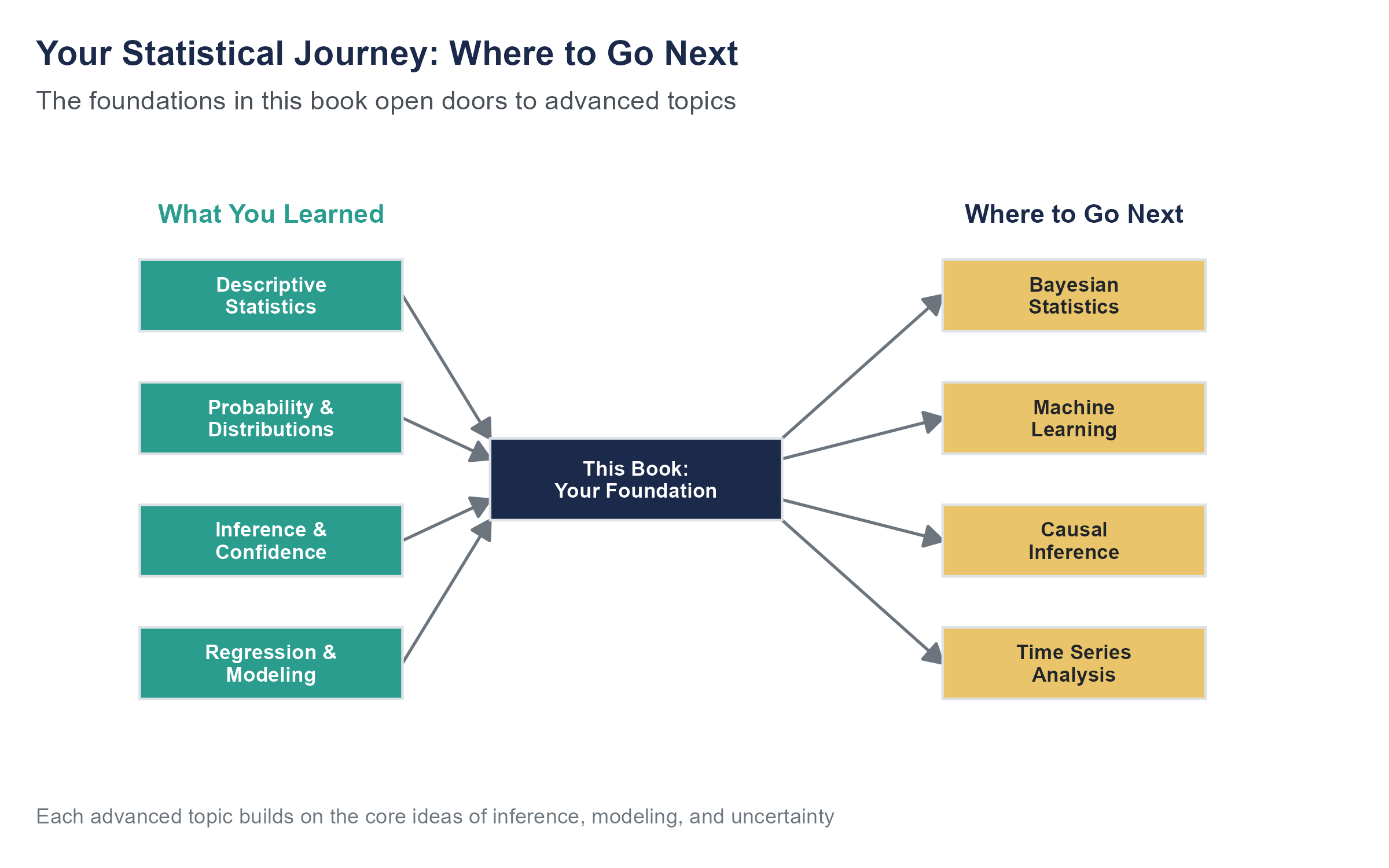
You have spent eleven chapters learning to think with data. You know how to design a study that can actually answer the question you care about. You know how to summarize information with numbers and pictures that do not mislead. You understand probability well enough to know that your intuitions about it are frequently wrong, and you know how to use the normal distribution and the central limit theorem to bridge the gap between a sample and a population. You can construct confidence intervals, test hypotheses, compare groups, and build regression models that separate signal from noise.
That is not a small thing. Most people who make decisions with data, in business, in government, in medicine, in everyday life, do not have even this much training. You are better equipped than you were twelve chapters ago, and better equipped than a large share of the people who will hand you charts and claim to know what the numbers mean.
But here is the honest truth. What you have learned is a foundation. A strong one, and one that will serve you well in a wide range of situations. But the field of statistics and data science extends far beyond what a single introductory course can cover. This chapter is about what lies ahead, not to overwhelm you, but to give you a sense of the terrain so you know where to go when you need more.
Think of it this way. You have learned to read. This chapter is a visit to the library.
12.2 Patterns Over Time
Every dataset we have worked with in this book treats each observation as independent, as if the order does not matter. Shuffle the rows of any dataset we have analyzed, and the results would come out the same. But in many real-world problems, order is everything. Stock prices tomorrow depend on stock prices today. Monthly sales figures follow seasonal rhythms. The number of emergency room visits fluctuates with day of the week, time of year, and whether there is a pandemic happening. Rearranging these observations would destroy the very structure that makes them informative.
Time series analysis is the branch of statistics that takes the clock seriously. Instead of treating time as just another variable, time series methods are built around the idea that what happened recently tells you something about what will happen next. The core concepts are trend (the long-run direction), seasonality (repeating patterns tied to calendar cycles), and noise (the unpredictable fluctuation that remains after you account for the other two). Models like ARIMA and exponential smoothing decompose a time series into these components and use the structure to generate forecasts.
If you have ever seen a weather forecast, an economic projection, or a demand planning model for a retail chain preparing for the holiday season, you have seen the output of time series analysis. The math gets involved, but the intuition is approachable. Past patterns, when understood carefully, help you anticipate the future.
To make this concrete, consider the problem of staffing an emergency department. Hospitals need to decide how many doctors, nurses, and support staff to schedule for each shift, every day, months in advance. Too few staff and patients wait dangerously long for care. Too many and the hospital wastes resources it cannot afford to waste. The solution is time series forecasting applied to patient arrival data. A good model captures the fact that Mondays are busier than Wednesdays, that flu season produces a predictable winter surge, that holidays bring spikes in certain types of injuries, and that a slow upward trend in the surrounding population means that last year’s staffing levels will not be enough this year. Each of those patterns (weekly seasonality, annual seasonality, holiday effects, long-run trend) can be modeled and projected forward. The forecasts are never perfect, because the noise component is real and irreducible. But they are far better than guessing, and in emergency medicine, the difference between a good forecast and a bad one is measured in lives.
The tricky part, and it is a hard part, is distinguishing patterns that will persist from patterns that are about to break. The financial crisis of 2008 was, among many other things, a failure of time series models that assumed housing prices would keep following the trend they had followed for decades. They did not. The models built on that assumption were not wrong about the past. They were catastrophically wrong about the future. The COVID-19 pandemic broke time series models across nearly every domain. Demand forecasts for retail, travel projections for airlines, energy consumption models for utilities, all of them relied on historical patterns that suddenly stopped applying. The models had no way to anticipate a once-in-a-century event because their entire logic depends on the future resembling the past. Understanding when to trust a forecast and when to question it is one of the deepest challenges in this area, and one of the reasons that human judgment remains essential even when the models are sophisticated.
12.3 Causation Gets Serious
In earlier chapters, we spent time on a distinction you will carry with you for the rest of your analytical life. Correlation is not causation. Observing that two variables move together does not mean one causes the other. We talked about confounders, omitted variables, and the dangers of drawing causal conclusions from observational data.
But here is the thing. Sometimes you need to know about causation, and you cannot run an experiment. You cannot randomly assign some cities to raise the minimum wage and others not to. You cannot randomly give some people health insurance and deny it to others, at least not without serious ethical guardrails. And yet policymakers need to know whether raising the minimum wage increases unemployment, and whether expanding health insurance improves health outcomes. The decisions will be made regardless. The question is whether they will be informed by credible evidence or by ideology and gut feeling.
A set of clever methods has emerged over the past few decades to tackle exactly this problem. They go by names like difference-in-differences, instrumental variables, and regression discontinuity, and they all share a common logic. If you cannot create a randomized experiment, look for situations in the real world that approximate one.
Difference-in-differences works by comparing two groups over two time periods. One group experiences some change (a new policy, a new program, an external shock) and the other does not. By comparing the before-and-after difference in the treatment group to the before-and-after difference in the comparison group, you can isolate the effect of the change from everything else that was happening at the same time. The classic example is the work of David Card and Alan Krueger on the minimum wage. In 1992, New Jersey raised its minimum wage while neighboring Pennsylvania did not. Card and Krueger surveyed fast-food restaurants on both sides of the border before and after the change, using Pennsylvania as a natural comparison group. Their analysis found no evidence that the minimum wage increase reduced employment, a finding that challenged decades of conventional economic wisdom and reshaped the entire debate. The study was controversial, and the debate continues, but the method itself opened a door that has never closed. David Card was awarded the Nobel Prize in Economics in 2021, in part for this and related empirical contributions to labor economics.
Regression discontinuity takes advantage of sharp cutoffs. If students who score above 80 on a test get a scholarship and students who score below 80 do not, then comparing students who scored 79 to students who scored 81 gives you something close to a randomized experiment, because the difference between those students is essentially random. The method is elegant precisely because it uses the arbitrariness of a threshold to create comparability.
Instrumental variables use a third variable to isolate variation in a cause that is unrelated to confounders. The logic is indirect and can be hard to grasp at first, but the method has been used to study questions ranging from the effect of education on earnings to the effect of military service on lifetime outcomes.
Another influential study in causal inference is the Oregon Health Insurance Experiment. In 2008, Oregon expanded its Medicaid program but had more applicants than slots, so it used a lottery to decide who received coverage. That lottery created something close to a randomized experiment at enormous scale, allowing researchers to study the causal effects of health insurance on health outcomes, financial security, and health care utilization with a rigor that observational data alone could never provide. The results were nuanced, showing clear improvements in financial security and mental health, but less clear effects on measured physical health outcomes, which itself became an important finding for the policy debate.
These methods are not magic. Each one relies on assumptions that must be argued for, not just asserted. Difference-in-differences requires that the two groups would have followed parallel trends without the intervention. Regression discontinuity requires that people cannot precisely manipulate their score to land on one side of the cutoff. Instrumental variables require that the instrument affects the outcome only through its effect on the treatment. Violate any of these assumptions, and the method falls apart. But if you find yourself in a career where you need to evaluate the effect of a policy, a program, or an intervention, this is the toolkit you will want next.
12.4 When Prediction Is the Point
Everything in this book has been oriented toward inference, toward understanding relationships, testing claims, and drawing conclusions about populations. But a parallel tradition in data analysis cares less about understanding and more about predicting. That tradition is machine learning.
The difference is subtle but important. In a regression model, you care about what the coefficients mean. Is the relationship between advertising spending and sales positive? How large is the effect? Is it statistically distinguishable from zero? In machine learning, you often do not care about interpreting individual parameters at all. You care about whether the model can accurately predict outcomes it has never seen before. A model that uses 500 variables in ways no human could interpret might be perfectly useful if your goal is to predict which customers will churn next month, which emails are spam, or which credit card transactions are fraudulent.
Machine learning encompasses a wide family of algorithms, from decision trees and random forests to neural networks and the deep learning models that power large language models like the one described in the AI Reality Checks throughout this book. Some of these methods have roots in the statistical methods you already know. Logistic regression, which you would encounter in a second statistics course, is also a core machine learning classifier. The lasso and ridge regression are extensions of the multiple regression you learned in Chapter 11, modified to handle situations with many more variables than observations.
One of the key ideas in machine learning is the distinction between training data and test data. When you fit a regression model in this book, you used all your data to estimate the coefficients. In machine learning, you typically split your data into two parts. You train the model on one part and evaluate its performance on the other part, data the model has never seen. This protects against overfitting, the problem of building a model that captures not just the real patterns in your data but also the noise, the random fluctuations that will not repeat in new data. A model that overfits looks great on the data it was trained on and performs terribly on new observations. If you have ever met someone who can explain everything that happened in the past but cannot predict anything about the future, you have met the human equivalent of an overfit model.
Here is a concrete example of how this plays out. In 2006, Netflix offered a million-dollar prize to anyone who could improve their movie recommendation algorithm by at least 10%. Thousands of teams competed over three years, building increasingly complex models that combined collaborative filtering (finding users who liked similar movies), matrix factorization, and ensemble methods that blended dozens of individual models together. The winning team, BellKor’s Pragmatic Chaos, achieved the 10% improvement target, but Netflix never fully implemented the winning solution. The model was too complex and too computationally expensive for production use, and by the time the prize was awarded, Netflix’s business had shifted from DVD rentals to streaming, which changed the prediction problem entirely. The competition remains a touchstone in the history of machine learning, not because the winning model was deployed, but because it demonstrated both the power and the practical limits of optimizing for prediction accuracy alone.
The tension between prediction and inference is a productive debate in modern data science. In many applications, you need both. You want a model that predicts well, and you want to understand why it predicts what it predicts. A hospital might use a machine learning model to predict which patients are at high risk of readmission, but doctors will not trust the model unless they can understand the factors driving those predictions. The field of interpretable machine learning has grown rapidly in response to this tension, developing tools that help explain the predictions of complex models. If this interests you, it is a productive area to explore next.
12.5 Updating Your Beliefs
Throughout this book, we have used the framework of frequentist statistics. Confidence intervals, hypothesis tests, p-values. These tools answer questions in a particular way. They ask, “If the null hypothesis were true, how surprising would this data be?” They do not directly tell you the probability that the null hypothesis is true, even though that is usually what you want to know.
Bayesian statistics offers a different framework, one that many people find more intuitive once they get past the initial unfamiliarity. The Bayesian approach starts with a prior, your best belief about a parameter before you see any data. Then you collect data, and the data updates your belief using Bayes’ theorem, producing a posterior, your revised belief that combines what you knew before with what the data tells you.
Here is a simple example. Suppose you are considering whether a coin is fair. Before flipping it, you believe it probably is, because most coins are fair. That is your prior. Then you flip it 20 times and get 15 heads. A frequentist approach would compute a p-value for the null hypothesis that the coin is fair. A Bayesian approach would combine your prior belief (probably fair) with the evidence (15 out of 20 heads) and give you a posterior distribution that shows how your belief has shifted. If your prior was strong, 20 flips might not move you much. If your prior was weak, the data will dominate.
Now consider a medical example. A diagnostic test for a rare disease comes back positive. If the disease affects 1 in 10,000 people and the test has a 5% false positive rate, then most positive results are false positives, a fact that remains stubbornly counterintuitive to most people, including many doctors. We covered this with Bayes’ theorem in the probability chapter. Bayesian statistics takes that same logic and extends it to every parameter you want to estimate, every hypothesis you want to evaluate, every prediction you want to make. It is Bayes’ theorem scaled up to the full range of statistical problems.
The Bayesian framework handles many problems more naturally than the frequentist one, especially problems involving sequential updating (you get more data over time and want to keep revising your estimate), incorporating expert knowledge, and making direct probability statements about hypotheses. It also avoids some of the interpretive headaches of p-values and confidence intervals. Instead of saying “we are 95% confident the parameter is in this interval” while carefully not saying “there is a 95% probability the parameter is in this interval,” a Bayesian analysis gives you a 95% credible interval that means exactly what you always wanted the confidence interval to mean. There is a 95% probability, given the data and the prior, that the parameter falls in this range. The trade-off is that it requires you to specify a prior, and people can disagree about what the right prior is, which introduces a layer of subjectivity that frequentist methods avoid, at least on the surface.
Consider a more consequential example. During the search for Malaysia Airlines Flight 370, which disappeared over the Indian Ocean in March 2014, analysts used Bayesian methods to guide the physical search. They started with a prior distribution over possible crash locations based on the flight’s last known position, fuel capacity, and satellite communication data. As search teams covered areas of ocean floor and found nothing, that absence of evidence became evidence itself. The posterior distribution was updated to shift probability away from searched areas and toward unsearched ones, focusing resources where the plane was most likely to be found given everything known so far. This sequential updating, where each new piece of information (including the information that a search area came up empty) refines the estimate, is Bayesian reasoning in its most natural form. The same approach had been used decades earlier to locate a lost hydrogen bomb off the coast of Spain in 1966 and to find the wreckage of the SS Central America in 1988. In each case, the Bayesian framework provided a principled way to combine incomplete information from multiple sources and update the search strategy as new data arrived.
Bayesian methods have become computationally practical thanks to advances in algorithms and computing power. Modern software like Stan and the brms package in R can fit complex Bayesian models that would have been impossible to compute a generation ago. If you continue in statistics or data science, you will eventually encounter Bayesian thinking, and when you do, you will find that the foundational concepts from this book, sampling distributions, estimation, the logic of evidence, translate directly.
12.6 The Responsibility You Carry
Let us turn from methods to something harder to put in a formula.
You now have tools that many people do not have. You can look at a dataset and see things that are invisible to someone without training. You can evaluate claims, check assumptions, identify misleading presentations of evidence, and construct analyses that separate real patterns from noise. These are powerful capabilities, and like all powerful capabilities, they can be used well or badly.
Data analysis is not neutral. Every choice an analyst makes, which variables to include, which observations to drop, which model to fit, which results to emphasize, shapes the conclusions that emerge. Two analysts working with the same data can reach different conclusions, not because one of them made an error, but because they made different defensible choices along the way. This is not a flaw in statistics. It is a feature of any discipline that requires judgment. But it means that the analyst’s integrity carries real weight.
Consider a few scenarios. A pharmaceutical company tests a drug in twelve subgroups and finds it works in one of them. They publish the positive result and do not mention the eleven failures. A consulting firm runs a regression with thirty potential control variables and reports the specification that makes the client’s product look best. A social media platform adjusts its engagement algorithm based on metrics that maximize time spent on the platform without measuring effects on users’ mental health. None of these involve fabricating data. All of them involve choices that distort the picture that data presents.
You will face situations where the data says something inconvenient. Where the results do not support the conclusion your boss wants, or the narrative your organization has already committed to, or the hypothesis you spent six months developing. In those moments, you will be tempted to go back and try different specifications, drop different outliers, reframe the question until the numbers cooperate. Some of that is legitimate exploratory analysis. Some of it is p-hacking, the practice the economist Ronald Coase called “torturing the data until it confesses,” which we discussed earlier in this book.
The line between legitimate exploration and data manipulation is not always bright, but here is a useful test. Would you be comfortable explaining every analytical choice you made to a skeptical but fair-minded colleague? If the answer is yes, you are probably on solid ground. If the answer involves phrases like “well, technically” or “it depends on how you look at it,” slow down.
This question of responsibility extends well beyond the classroom. Consider how it plays out in something as everyday as a lending algorithm. Having the technical ability to build a model does not, by itself, tell you whether the model should be built, or how it should be used, or who bears the cost when it is wrong. A lending algorithm that maximizes profit for the lender while systematically disadvantaging certain communities might score well on traditional accuracy metrics and still be doing harm. The statistical question, “does this model predict accurately?”, is necessary but not sufficient. You also need to ask who benefits, who is harmed, and whether the trade-offs are justified.
Those are questions that require judgment and an awareness of how the model’s outputs land on the people they describe. Analyzing data is one skill. Asking whether an analysis is being used responsibly is a second skill, and the second is at least as worth developing as the first. You are now in a position to do both.
We have included AI Reality Checks throughout this book, and this one is the last, so it is worth making count.
Artificial intelligence, and large language models in particular, will keep getting better at computation. They can already clean data, run regressions, generate visualizations, write code, and summarize findings faster than any human. By the time you read this, they will probably be even better at all of those things. The trajectory is clear, and it would be foolish to pretend otherwise.
But computation is not the hard part. The hard part is deciding what computation to run. The hard part is knowing whether a regression model is appropriate or whether the data violates the assumptions in ways that make the output misleading. The hard part is recognizing when a question sounds statistical but is actually ethical, or political, or deeply contextual in ways that no model can resolve on its own. The hard part is having the judgment to say “this analysis answers the wrong question” when everyone around you is excited about the results.
AI will not replace the person who can think critically about data. It will replace the person who cannot. If all you know is how to plug numbers into formulas and report the output, you are competing with software that does it faster and cheaper. If you know how to frame questions, evaluate assumptions, interpret results in context, communicate uncertainty honestly, and exercise judgment about what the numbers mean for real people, you are the person the AI needs on the other end of the conversation.
Here is a concrete way to think about it. An AI can build you a regression model in seconds. It can test every possible combination of variables, try dozens of functional forms, and report the one with the best fit statistics. What it cannot do, at least not yet, is sit with a community group and understand why a particular variable should not be used as a predictor even though it improves accuracy. It cannot navigate the trade-off between a model that is slightly less predictive and one that is fairer. It cannot decide whether a finding should be published or whether doing so would cause more harm than good. Those decisions require something the model does not have.
Your job, going forward, is not to be the computer. Your job is to be the person who asks whether the computation was the right one to run.
12.7 The Statistical Mindset
Before we turn to resources and reading lists, I want to pause and talk about something that does not fit neatly into any single chapter but runs through all of them. Call it the statistical mindset. It is the collection of habits, instincts, and reflexes that you have been building throughout this book, and it is arguably more valuable than any individual technique you have learned.
The statistical mindset begins with a comfort with uncertainty. Most of the decisions you will face in your life, in your career, in your community, in your personal choices, will be made with incomplete information. You will never have the whole picture. You will never be able to eliminate all the confounders, survey the entire population, or predict the future with certainty. The statistical mindset does not pretend otherwise. Instead, it asks a different question. Given what I know (and what I do not know), what is the most reasonable conclusion? How confident should I be? What would change my mind?
That last question is particularly important. One of the most underrated skills in analytical thinking is the ability to specify, in advance, what evidence would cause you to revise your position. If the answer is “nothing,” you are not reasoning. You are advocating. There is a place for advocacy, but it is not the same thing as analysis, and confusing the two is a common mistake people make when working with data.
The statistical mindset also involves a habit of asking “compared to what?” Every number, every result, every trend exists in context. A company reporting 10% revenue growth sounds impressive until you learn that the industry grew 25% over the same period. A medical treatment that reduces the risk of a disease by 50% sounds like a breakthrough until you learn that the risk went from 2 in 10,000 to 1 in 10,000. An absolute difference that small might not justify the cost and side effects of the treatment. You learned about this distinction between relative and absolute differences earlier in the book, and it is an idea worth keeping close. Once you start asking “compared to what?” you cannot stop. It changes how you read news, how you evaluate marketing claims, and how you think about your own experiences.
Another piece of the statistical mindset is a respect for variation. Before this book, you might have thought of an average as a fact, a single number that captures the truth about a group. Now you know better. An average is a summary, and like all summaries, it leaves things out. The distribution behind the average matters. The spread matters. The shape matters. Two groups can have the same average and look completely different. A single outlier can drag a mean in a misleading direction. When someone gives you an average without telling you about the variation, you now know to be suspicious, and that suspicion is well-calibrated.
There is also the habit of thinking about how data was generated. This is one of the first things a trained analyst does when encountering a new dataset, and it is one of the last things an untrained one thinks to ask. Where did this data come from? Who collected it? How were the participants or observations selected? What is missing? The answers to these questions determine what conclusions the data can support, regardless of how fancy the analysis is. A machine learning model trained on biased data will produce biased predictions, and no amount of algorithmic sophistication will fix a sampling problem. You learned this in Chapter 2 when we discussed study design, and it applies to every analysis you will ever encounter.
Finally, the statistical mindset includes a willingness to say “I do not know.” This might be the hardest habit to develop, because the world rewards confidence and penalizes uncertainty. People who say “the data is inconclusive” get less attention than people who say “the data proves X.” Analysts who report wide confidence intervals feel less useful than analysts who report narrow ones. But honest uncertainty is more valuable than false precision. A confidence interval that is wide because the sample was small is telling you something important. Ignoring that message, or hiding it behind false certainty, leads to bad decisions. The statistical mindset treats uncertainty not as a failure but as information, something to be quantified, communicated, and respected.
You may not realize it yet, but these habits have already started to change how you think. The next time someone shows you a chart without axes, you will notice. The next time someone claims a causal relationship based on a correlation, you will hesitate. The next time you hear a news story about a study that “proves” something, you will want to know the sample size, the confidence interval, and whether the result has been replicated. These are more than academic reflexes. They are practical tools for navigating a world that produces more data than understanding.
The formal techniques in this book, the confidence intervals and hypothesis tests and regression models, are important. But they are tools. The statistical mindset is what tells you which tool to pick up, when to put it down, and what to do when no tool quite fits the problem in front of you. Carry it with you. It will serve you well in places you do not yet expect.
If you have made it this far, through all twelve chapters, through the formulas and the examples and the careful distinctions between what data can and cannot tell you, then you have done something that matters. You have learned to think more carefully about evidence. You have built a set of tools for reasoning under uncertainty. And you have, I hope, developed a healthy respect for both the power and the limits of statistical analysis.
The world is full of numbers. They show up in news headlines, in business dashboards, in medical studies, in policy debates, in the algorithms that shape what you see and buy and believe. Some of those numbers are presented honestly. Some are not. Some are analyzed well. Some are not. Before this book, you might not have been able to tell the difference. Now you can, or at least you can start to, and that changes things.
I want to leave you with one thought. Statistics is often taught as if it were a finished product, a set of techniques to be memorized and applied. It is not. It is a living discipline, constantly evolving, constantly arguing with itself about the right way to reason from evidence. The debates between frequentists and Bayesians, between prediction and inference, between complexity and interpretability, are not signs of a field in trouble. They are signs of a field that takes its own questions seriously. As you move forward, I hope you will engage with those questions, beyond being a consumer of statistical results, as someone who contributes to better thinking about data in whatever context you find yourself.
12.8 Where to Keep Learning
This book has given you a foundation, but a foundation is only useful if you build on it. Here are resources for the directions discussed in this chapter, drawn from books that have shaped how working analysts and researchers think about each topic.
For machine learning. An Introduction to Statistical Learning by Gareth James, Daniela Witten, Trevor Hastie, and Robert Tibshirani is the best bridge between the statistics you have learned here and the world of machine learning. It is rigorous without being inaccessible, and it is available as a free PDF from the authors’ website. The book covers classification, resampling methods, tree-based models, support vector machines, and unsupervised learning, all building on the regression foundation you developed in Chapters 10 and 11. What makes this book special is that it was written by statisticians for a broad audience, so the emphasis is on concepts and applications rather than mathematical proofs. It has become a standard textbook in data science.
For causal inference. Two outstanding books are available for free online. Causal Inference: The Mixtape by Scott Cunningham covers the methods I described earlier in this chapter, difference-in-differences, instrumental variables, regression discontinuity, and more, with clear explanations and code examples in both Stata and R. Cunningham writes with personality and wit, which makes the sometimes-dense material more approachable than you might expect. The Effect: An Introduction to Research Design and Causality by Nick Huntington-Klein takes a similar approach with a slightly different emphasis, excellent visualizations, and code in R, Python, and Stata. Huntington-Klein is particularly good at using diagrams and directed acyclic graphs (DAGs) to make causal reasoning visual and intuitive. Either one would be a natural next step from this book.
For Bayesian statistics. Statistical Rethinking by Richard McElreath is the book I would recommend starting with. McElreath writes with unusual clarity, and the accompanying lecture videos (freely available online) are some of the best statistics teaching I have encountered in any format. The book takes a fundamentally Bayesian approach to statistical modeling and will change how you think about many of the methods covered in this textbook. For a more comprehensive and advanced treatment, Bayesian Data Analysis by Andrew Gelman, John Carlin, Hal Stern, David Dunson, Aki Vehtari, and Donald Rubin is the standard reference. I would recommend tackling Gelman after you have taken at least one more statistics course, but if Bayesian thinking intrigues you, even reading the first few chapters of either book will deepen your understanding of how statistical reasoning works and why the frequentist-Bayesian debate matters.
For time series. Forecasting: Principles and Practice by Rob Hyndman and George Athanasopoulos is available free online and is, in my opinion, one of the best-written statistics textbooks in any subfield. Hyndman is one of the leading researchers in forecasting, and the book covers everything from simple exponential smoothing to modern methods like ARIMA and dynamic regression. The R code is integrated throughout, so you can work through the examples as you read. If the time series section of this chapter sparked your curiosity, this is the place to go.
For critical thinking about data. Calling Bullshit: The Art of Skepticism in a Data-Driven World by Carl Bergstrom and Jevin West is the book I wish everyone would read. It is not a statistics textbook. It is a book about how data, statistics, and quantitative arguments are used to mislead, sometimes intentionally and sometimes not, and how to defend yourself against it. The authors cover misleading visualizations, selection bias in big data, the misuse of algorithms, and the way that quantitative claims acquire unearned authority simply by being quantitative. It pairs beautifully with the skills you have developed in this book, and it is the rare book that will make you both smarter and more humble about how much you do not know.
12.9 Parting Words
We started this book in Flint, Michigan, where the water was poisoned and the people who said so were told they were wrong. Marc Edwards and Mona Hanna-Attisha did not uncover the Flint water crisis with fancy algorithms or advanced methods. They used the same basic tools you have spent this book learning. Sampling. Distributions. Comparisons between groups. Confidence in their data and the courage to present it clearly when the people in power did not want to hear it.
What made the difference in Flint was not the sophistication of the statistics. It was the fact that someone knew how to ask the right question, collect the right data, analyze it honestly, and stand behind the results. Edwards looked at the distribution of lead levels across hundreds of homes and saw a pattern that could not be explained away. Hanna-Attisha compared blood lead levels before and after the water switch and found a difference that was too large and too consistent to be coincidence. These are not exotic techniques. They are the methods you learned in the first half of this book.
That is both the humbling and the hopeful message of this book. The tools are not complicated. What is rare is the willingness to use them honestly, the discipline to follow the evidence where it leads, and the willingness to stand behind findings even when they are inconvenient. Flint needed someone who could look at data and see what it contained. Your community, your workplace, your corner of the world, needs people like that too.
You now have the foundation to be one of them. Not because you have memorized every formula in this book (you will forget most of them, and that is fine, because you can always look them up). But because you understand what the formulas are for. You understand that data does not speak for itself. It speaks through the people who collect it, analyze it, and interpret it with care. You understand that uncertainty is not weakness but honesty, that a well-constructed confidence interval is more valuable than a false certainty, and that the gap between what the data says and what someone claims the data says is often where the most important work happens.
It has been a privilege to guide you through this material. Whatever direction you go from here, you carry with you a set of ideas that will help you see the world more clearly, ask better questions, and reach better-supported conclusions. That was always the point.
Thank you for reading.
12.10 References
Bergstrom, C. T., & West, J. D. (2020). Calling bullshit: The art of skepticism in a data-driven world. Random House.
Card, D., & Krueger, A. B. (1994). Minimum wages and employment: A case study of the fast-food industry in New Jersey and Pennsylvania. American Economic Review, 84(4), 772-793.
Cunningham, S. (2021). Causal inference: The mixtape. Yale University Press.
Davey, S. J., Gordon, N., Holland, I. D., Rutten, M., & Williams, J. (2016). Bayesian methods in the search for MH370. Springer. (A detailed account of how Bayesian updating guided the physical search for Malaysia Airlines Flight 370, the application described in this chapter’s section on Bayesian statistics.)
Finkelstein, A., Taubman, S., Wright, B., Bernstein, M., Gruber, J., Newhouse, J. P., Allen, H., Baicker, K., & Oregon Health Study Group. (2012). The Oregon Health Insurance Experiment: Evidence from the first year. Quarterly Journal of Economics, 127(3), 1057-1106.
Gelman, A., Carlin, J. B., Stern, H. S., Dunson, D. B., Vehtari, A., & Rubin, D. B. (2013). Bayesian data analysis (3rd ed.). Chapman and Hall/CRC.
Huntington-Klein, N. (2021). The effect: An introduction to research design and causality. Chapman and Hall/CRC.
Hyndman, R. J., & Athanasopoulos, G. (2021). Forecasting: Principles and practice (3rd ed.). OTexts.
James, G., Witten, D., Hastie, T., & Tibshirani, R. (2021). An introduction to statistical learning: With applications in R (2nd ed.). Springer.
McElreath, R. (2020). Statistical rethinking: A Bayesian course with examples in R and Stan (2nd ed.). CRC Press.
McGrayne, S. B. (2011). The theory that would not die: How Bayes’ rule cracked the Enigma code, hunted down Russian submarines, and emerged triumphant from two centuries of controversy. Yale University Press. (A narrative history of Bayesian reasoning covering the Palomares hydrogen bomb search and the SS Central America discovery discussed in this chapter, accessible to a general audience.)