8 Hypothesis Testing

8.1 Did It Actually Work?

In 2007, a company called Opower began partnering with electric utilities across the United States to send home energy reports to residential customers. The reports were simple. Each household received a letter showing how much electricity it used compared to its neighbors, complete with smiley faces for efficient homes and gentle nudges for the less efficient ones. The idea drew on decades of behavioral science research suggesting that social comparisons can motivate people to change their behavior. If you knew that your neighbors were using less electricity than you, the theory went, you might turn off a few lights, adjust your thermostat, or replace that ancient refrigerator.

The program was a nonprofit’s dream, a low-cost intervention that could scale to millions of households. But before anyone invested further, there was a question that needed answering.

Did it work?

That question is harder than it sounds.

Hunt Allcott, an economist then at NYU, set out to answer it rigorously. He studied Opower’s program across multiple utility companies serving hundreds of thousands of households. The study design was careful. In each utility service area, households were randomly assigned to either receive the energy reports (the treatment group) or not receive them (the control group). Then Allcott compared electricity usage between the two groups over time.

The data showed that households receiving the reports used, on average, about 2% less electricity than households in the control group. Two percent. That was the number.

Now, two reactions are possible here. The first is to shrug. Two percent sounds small. Is it even worth the cost of printing and mailing all those reports? The second reaction is to ask a more fundamental question, one that comes before any discussion of whether the effect is big enough to care about.

Is the difference real?

Those households that got the reports used 2% less energy, on average, than those that did not. But averages vary from sample to sample. Even if the reports had absolutely zero effect on behavior, you would not expect the treatment and control groups to use exactly the same amount of electricity. Random variation alone would produce some difference. Maybe the treatment group just happened to include more naturally frugal people. Maybe the weather was different in the areas where reports were delivered. Maybe the 2% difference is nothing more than the kind of random fluctuation you would expect even if the reports did absolutely nothing.

This is the question that hypothesis testing was built to answer. Not “is the effect big enough to matter” (that comes later), but “is there an effect at all, or are we fooling ourselves?”

Allcott’s analysis concluded that the effect was real and very unlikely to have arisen by chance alone. His 2011 paper, published in the Journal of Public Economics, became widely cited in behavioral economics. The Opower program went on to reach more than 50 million households, and the company was acquired by Oracle in 2016. But to understand why Allcott’s conclusion was justified, and when similar conclusions are not, you need to understand the logic, machinery, and limitations of hypothesis testing.

That is what this chapter is about. It is also the densest chapter in this book, and the one whose ideas show up most often in subsequent chapters.

8.2 The Logic of Hypothesis Testing

8.2.1 Starting with a Question

Every hypothesis test begins with a question about a population. Does this drug lower blood pressure? Do customers who see the redesigned website buy more? Did the energy reports reduce electricity consumption?

We cannot observe the entire population, so we collect data from a sample and use that sample to make an inference about the population. We have been building toward this since Chapter 1. Hypothesis testing formalizes the process by forcing us to state our question precisely, collect evidence, and evaluate that evidence against a specific standard.

8.2.2 Null and Alternative Hypotheses

The formal framework requires two competing statements.

The null hypothesis, written $H_0$, is the default position. It states that nothing interesting is happening, that there is no effect, no difference, no relationship. In the Opower example, the null hypothesis would be that the energy reports have no effect on electricity usage, that the true mean difference in consumption between the treatment and control groups is zero.

\[H_0: \mu_{\text{treatment}} - \mu_{\text{control}} = 0\]

The alternative hypothesis, written $H_a$ (or sometimes $H_1$), is the claim that something is going on. It states that there is an effect, a difference, a relationship. For Opower, the alternative hypothesis is that the reports do change electricity consumption.

\[H_a: \mu_{\text{treatment}} - \mu_{\text{control}} \neq 0\]

Notice the structure. The null hypothesis is specific (the difference is exactly zero), while the alternative hypothesis is broad (the difference is anything other than zero). This asymmetry is deliberate and important. We do not try to prove the alternative hypothesis. Instead, we ask whether the data provides enough evidence to reject the null hypothesis. The burden of proof falls on the claim that something is happening.

8.2.3 The Courtroom Analogy

The most common way to explain this logic is through a courtroom analogy, and it is useful enough to walk through, even though it has limitations we should be honest about.

In a criminal trial in the United States, a defendant is presumed innocent until proven guilty. The prosecution must present evidence beyond a reasonable doubt to convince the jury to convict. If the evidence is insufficient, the jury returns a verdict of “not guilty.” Note that “not guilty” is not the same as “innocent.” It means the prosecution failed to meet its burden.

Hypothesis testing follows a similar structure.

The null hypothesis ($H_0$) is like the presumption of innocence. It stands unless the evidence overturns it.
The alternative hypothesis ($H_a$) is like the prosecution’s claim that the defendant is guilty.
The data is the evidence presented at trial.
The p-value (which we will define shortly) measures the strength of the evidence against the null hypothesis.
Rejecting $H_0$ is like a guilty verdict. We have enough evidence to act on the claim.
Failing to reject $H_0$ is like a not guilty verdict. We do not have enough evidence to reject the default position.

This analogy captures the key asymmetry. We never “accept” the null hypothesis, just as a jury never declares a defendant innocent. We either reject it or we fail to reject it. The absence of evidence against the null is not the same as evidence for the null.

Note

The phrasing “fail to reject $H_0$” sounds awkward, and students sometimes wonder why we do not just say “accept $H_0$.” The reason matters. Failing to reject $H_0$ means we did not find enough evidence against it. Maybe the null is true. Or maybe there is an effect, but our sample was too small to detect it, or our measurement was too noisy. We simply cannot tell. Saying “accept $H_0$” implies a confidence we do not have.

8.2.4 Where the Analogy Breaks Down

The courtroom analogy is helpful but imperfect, and glossing over its limitations leads to misunderstanding.

First, criminal trials use “beyond a reasonable doubt” as the standard. Hypothesis testing uses a numerical significance threshold — almost always 5% — which is a much lower bar than what a criminal court would accept. In a criminal trial, we tolerate a high standard because convicting an innocent person is a serious error. In statistics, the threshold depends on context, and the 5% level is a convention, not a law of nature. We will define this threshold formally as $\alpha$ in just a moment.

Second, juries weigh qualitative evidence, witness credibility, narratives, and context. Hypothesis testing reduces the evidence to a single number (the p-value). Important context can get lost in that reduction.

Third, and most critically, the courtroom analogy encourages binary thinking, guilty or not guilty, reject or fail to reject. But the strength of evidence exists on a continuum. A p-value of 0.049 and a p-value of 0.051 are practically identical, yet one crosses a conventional threshold and the other does not. Treating these as fundamentally different is one of the most persistent problems in statistical practice.

We will return to this problem. For now, let us look at how the evidence is actually measured.

8.3 Test Statistics and P-Values

8.3.1 The Test Statistic

Suppose you want to test whether a coin is fair. You flip it 100 times and get 58 heads. Is the coin biased? Your sample proportion is 0.58, which is not 0.50, but samples vary. Even a perfectly fair coin would not give exactly 50 heads every time.

The question is whether 58 heads out of 100 is unusual enough to cast doubt on the claim that the coin is fair. To answer that, we need to quantify “unusual enough.”

A test statistic is a number that measures how far our sample result falls from what the null hypothesis predicts. The specific formula depends on the type of test, but the logic is always the same. The test statistic captures the discrepancy between what we observed and what we would expect if $H_0$ were true, scaled by how much variability we would expect in our samples.

In its most general form, a test statistic looks like this:

\[\text{Test Statistic} = \frac{\text{Observed value} - \text{Expected value under } H_0}{\text{Standard error}}\]

A large test statistic (far from zero) means the data is far from what the null hypothesis predicts. A small test statistic (close to zero) means the data is consistent with the null.

Which Do I Need: SD or SE?

Standard deviation (SD) describes how much individual observations vary around the mean. It tells you about the spread in your data.

Standard error (SE) describes how much a sample statistic (like the mean) would vary if you repeated the study. It tells you about the precision of your estimate.

Use SD when describing your data. Use SE when making inferences about a population.

Figure 8.1: The null distribution (standard normal) with two-tailed rejection regions shaded in coral. A test statistic of z = 2.3 falls in the rejection region beyond the critical value of 1.96, leading to rejection of the null hypothesis at the 0.05 significance level.

8.3.2 What Is a P-Value?

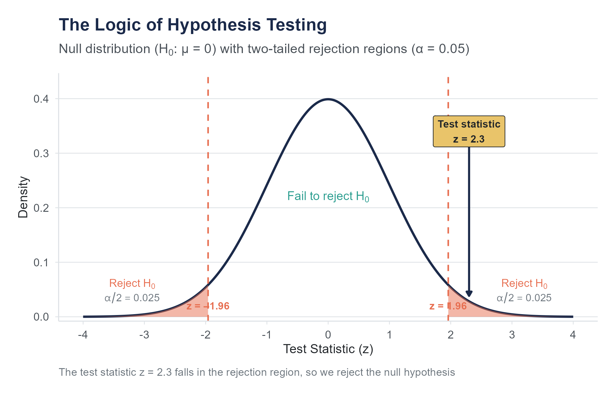
The p-value is the probability of observing a test statistic as extreme as, or more extreme than, the one we actually calculated, assuming the null hypothesis is true.

Read that definition again. Slowly. It is a specific, technical definition, and every word matters. Many smart people get this wrong, and the consequences of getting it wrong are not academic.

The p-value answers this question: “If there were truly no effect (if $H_0$ were true), how likely would we be to see data at least this extreme?”

Think of it this way. Imagine you could rerun the study thousands of times in a universe where $H_0$ is true, where the treatment has no effect at all. In some of those repetitions, you would see small differences between groups. In a few, you would see larger differences, purely by luck. The p-value tells you what fraction of those repetitions would produce a result as extreme or more extreme than what you actually observed.

If the p-value is very small, it means that data like ours would be very unlikely under the null hypothesis. We take this as evidence against the null. If the p-value is not small, it means that data like ours would be quite plausible even if there were no effect. In that case, we have no compelling reason to reject the null.

For the coin example, the p-value would answer this: “If the coin were perfectly fair, what is the probability of getting 58 or more heads (or 42 or fewer) in 100 flips?” If that probability is very low, we have reason to suspect the coin is not fair.

8.3.3 The Significance Level

We need a threshold for “small enough.” The significance level, denoted $\alpha$ (alpha), is the probability threshold below which we reject $H_0$. By convention, $\alpha = 0.05$ is the most common choice, meaning we reject the null hypothesis if the p-value is less than 0.05.

If that number looks familiar, it should. In Chapter 7, the same value appeared from the other side: a 95% confidence level corresponds to an $\alpha$ of $1 - 0.95 = 0.05$. Confidence intervals and hypothesis tests are using the same dial, just labeled differently. A two-sided test at level $\alpha$ rejects $H_0$ for exactly the values that fall outside a $(1 - \alpha)$ confidence interval.

The decision rule is straightforward:

If $p \leq \alpha$, reject $H_0$. The result is “statistically significant.”
If $p > \alpha$, fail to reject $H_0$. The result is “not statistically significant.”

Where did 0.05 come from? Ronald Fisher introduced it in his 1925 book Statistical Methods for Research Workers, where he proposed the 5% level as a convenient cutoff — “1 in 20 chance of being exceeded by chance.” Fisher framed it as a rule of thumb rather than a strict rule, and later in his career he was clearer that the threshold should depend on context. There is nothing magical about it. In some fields, a stricter threshold is standard (particle physics uses roughly $\alpha = 0.0000003$, or “five sigma,” before claiming a discovery). In others, a more relaxed threshold might be appropriate. The choice of $\alpha$ should be made before looking at the data and should reflect the consequences of making the wrong decision.

Note

In 2018, a group of 72 prominent researchers published a paper in Nature Human Behaviour proposing that the default significance threshold be lowered from 0.05 to 0.005 for claims of new discoveries. Their argument was that the 0.05 threshold produces too many false positives, contributing to the replication crisis. The proposal sparked intense debate and has not been universally adopted, but it highlights that the choice of $\alpha$ is a judgment call with real consequences for science.

8.3.4 What a P-Value Is NOT

The p-value is one of the most misunderstood concepts in all of statistics. Here are the most common misinterpretations, all of them wrong.

Wrong: “The p-value is the probability that the null hypothesis is true.” No. The p-value is calculated assuming the null hypothesis is true. It cannot tell you the probability that $H_0$ is true or false. That would require a fundamentally different framework (Bayesian statistics, which we touch on in Chapter 12).

Wrong: “A p-value of 0.03 means there is a 3% chance the results are due to chance.” This sounds close to the correct definition but subtly reverses the logic. The p-value is the probability of the data given the null, not the probability of the null given the data. These are not the same thing, just as the probability that a dog has four legs is not the same as the probability that a four-legged creature is a dog.

Wrong: “A smaller p-value means a bigger effect.” No. A tiny p-value can come from a huge effect in a small sample or from a tiny effect in a huge sample. The p-value mixes together the size of the effect and the size of the sample. To understand the size of the effect, you need a different measure (which we will cover shortly).

Wrong: “A p-value greater than 0.05 means there is no effect.” No. It means we did not find sufficient evidence against the null hypothesis. As Carl Sagan put it, the absence of evidence is not evidence of absence. The effect might exist but be too small for our sample to detect.

Wrong: “A p-value of 0.05 means the result has a 95% chance of being correct.” No. This confuses the p-value with the confidence level and misinterprets both.

If you take nothing else from this section, take this: a p-value is a measure of the compatibility between the data and a specific null hypothesis. It is not a measure of truth, importance, or certainty.

8.4 Type I and Type II Errors

When we make a decision about $H_0$, we can be right or we can be wrong, and there are exactly two ways to be wrong.

8.4.1 Type I Error (False Positive)

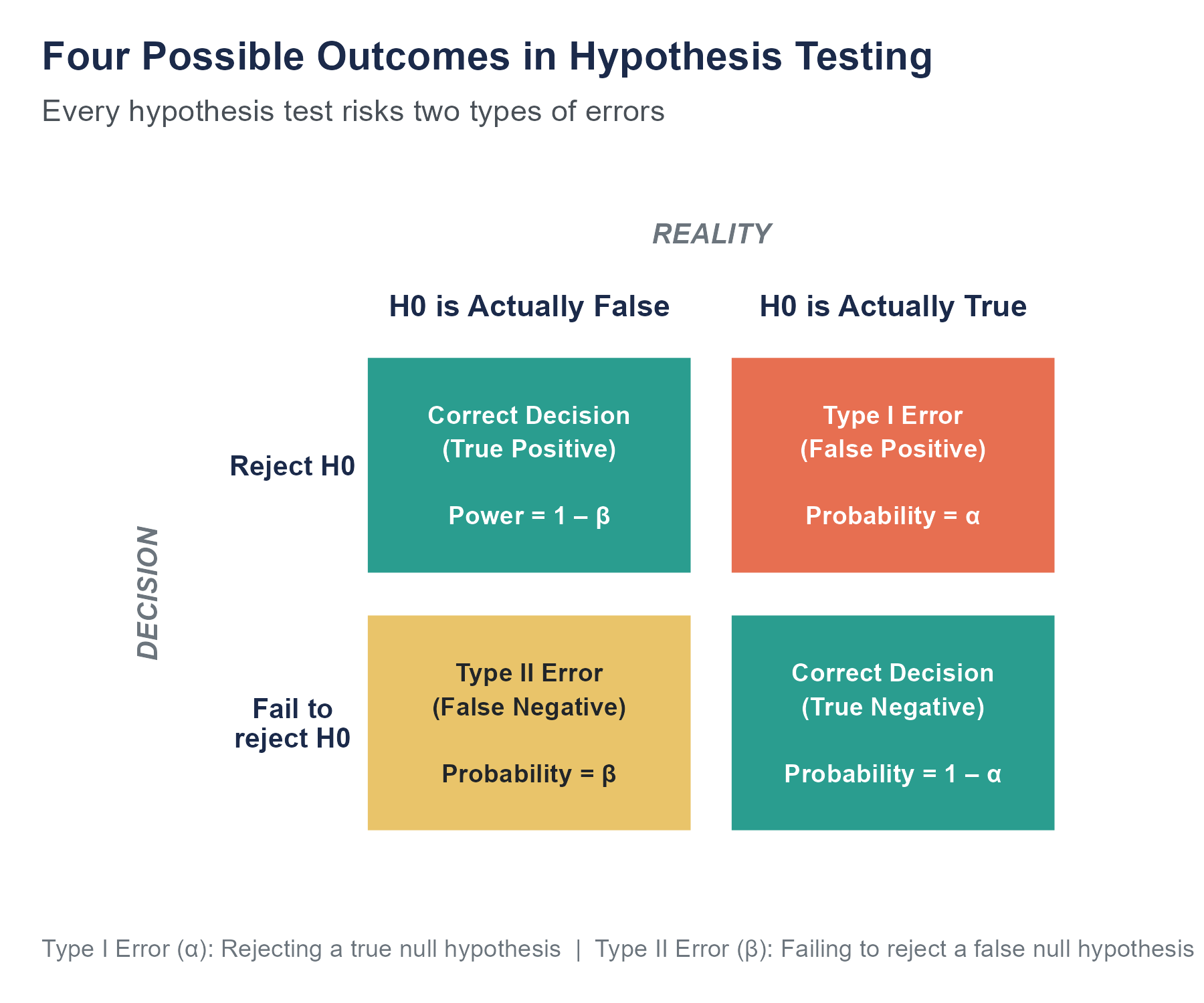
A Type I error occurs when we reject $H_0$ even though it is actually true. We conclude there is an effect when there is not one. This is a false alarm.

The probability of a Type I error is $\alpha$, the significance level we chose. When we set $\alpha = 0.05$, we are accepting a 5% chance that we will reject a true null hypothesis. This is not a bug in the system; it is a conscious tradeoff. We accept some risk of false positives in order to have a reasonable chance of detecting real effects.

8.4.2 Type II Error (False Negative)

A Type II error occurs when we fail to reject $H_0$ even though it is actually false. There is a real effect, but we missed it. This is a miss.

The probability of a Type II error is denoted $\beta$ (beta). Unlike $\alpha$, which we set in advance, $\beta$ depends on several factors: how big the true effect is, how large our sample is, and how much variability there is in the data.

8.4.3 Power

Power is the probability of correctly rejecting a false null hypothesis. It is the complement of $\beta$:

\[\text{Power} = 1 - \beta\]

Power is the probability of detecting an effect that actually exists. A study with low power is like a metal detector with a weak signal: even if there is something buried there, you might walk right over it and hear nothing.

What determines power?

Effect size. Bigger effects are easier to detect. A drug that lowers blood pressure by 20 points is easier to detect than one that lowers it by 2 points.
Sample size. Larger samples give more precise estimates, making it easier to distinguish a real effect from noise.
Variability. Less variability in the data (smaller standard deviations) makes effects easier to detect.
Significance level. A more lenient $\alpha$ (say, 0.10 instead of 0.05) increases power but also increases the risk of Type I error. You cannot reduce both error types simultaneously without increasing sample size.

A common target for power is 0.80 (80%), meaning an 80% chance of detecting the effect if it exists. This is a convention, not a rule. For high-stakes studies, higher power might be warranted. For preliminary or exploratory work, lower power might be acceptable.

8.4.4 Why Power Matters in Practice

Underpowered studies are a recurring problem in published research, with consequences that reach beyond the academic literature. An underpowered study is one with too small a sample to have a reasonable chance of detecting the effect it is looking for. These studies are common. A review by Button and colleagues (2013) found that the median neuroscience study had statistical power of about 21% — only a 1 in 5 chance of detecting a real effect. Studies like these were unlikely to produce a significant result from the start, even when the underlying effect was real.

This creates two problems. First, the non-significant results are uninformative: we cannot tell whether the treatment did not work or whether the study was just too small to tell. Second, and more insidiously, the studies that do manage to find significant results in underpowered conditions are likely to be overestimates of the true effect size. This is because only the studies where random variation happened to inflate the effect will cross the significance threshold. It is a selection effect. The published literature ends up populated with inflated effects that fail to replicate, which is exactly what the replication crisis looks like from the inside.

The solution is simple in theory, if sometimes difficult in practice. Before you run a study, do a power analysis. Determine how large a sample you need to have a reasonable chance of detecting the smallest effect you would consider important. If you cannot afford a sample that large, be honest about the limitations of your study rather than running it anyway and treating a non-significant result as evidence that nothing is going on.

The following table summarizes the four possible outcomes:

	$H_0$ is True	$H_0$ is False
Reject $H_0$	Type I Error ($\alpha$)	Correct Decision (Power = $1-\beta$)
Fail to Reject $H_0$	Correct Decision ($1-\alpha$)	Type II Error ($\beta$)

Think of it this way. Lowering $\alpha$ reduces your risk of false positives but increases your risk of false negatives. You become harder to fool, but you also become more likely to miss real effects. The only free lunch is a bigger sample, which reduces both error rates simultaneously.

Figure 8.2: A 2x2 grid showing the four possible outcomes in hypothesis testing. Correct decisions appear on the diagonal (true positive with power = 1 minus beta, and true negative with probability 1 minus alpha), while errors appear off the diagonal (Type I error with probability alpha, and Type II error with probability beta).

Try It Online

Explore how sample size, effect size, and significance level affect power using the Hypothesis Testing Playground. Increase the sample size and watch the power curve shift. Then change the true effect size and see how the overlap between the null and alternative distributions changes.

8.5 Statistical Significance vs. Practical Significance

This is where many analysts, journalists, and even researchers go wrong.

A result is statistically significant if the p-value is below the chosen $\alpha$ threshold. That tells you the observed difference is unlikely to be entirely due to random chance. It does not tell you the difference is big, important, or worth acting on.

Return to the Opower study. The energy reports produced a statistically significant reduction in electricity consumption. The p-value was far below 0.05. But the effect size was about 2%. Two percent. Is that practically meaningful?

That depends on context. For an individual household, saving 2% on an electricity bill might be barely noticeable. But across millions of households, a 2% reduction aggregates to enormous energy savings, reduced carbon emissions, and measurable environmental impact. Practical significance depends on the scale and context of the application, beyond whether a p-value crossed a threshold.

8.5.1 The Large-Sample Problem

Here is an underappreciated fact. With a large enough sample, you can find statistically significant results for differences so tiny they are meaningless.

Suppose a company tests two versions of a website button, blue vs. green, and 500,000 people see each version. The blue button has a click rate of 3.01% and the green button has a click rate of 3.00%. With half a million people in each group, this 0.01 percentage point difference could easily produce a p-value below 0.05. Statistically significant. But is a company going to redesign its website over a difference of one click per ten thousand visitors? It should not.

Conversely, a small study might observe a large and practically important difference, say a 15-point reduction in blood pressure, but fail to reach statistical significance because the sample was too small and the uncertainty too wide.

Statistical significance and practical significance are different things. You need to assess both.

8.5.2 Effect Sizes

An effect size is a standardized measure of how large a difference or relationship is, independent of sample size.

The most common effect size for comparing two means is Cohen’s d:

\[d = \frac{\bar{x}_1 - \bar{x}_2}{s_p}\]

where $\bar{x}_1$ and $\bar{x}_2$ are the sample means and $s_p$ is the pooled standard deviation. Cohen’s d tells you how many standard deviations apart the two group means are.

Jacob Cohen proposed rough benchmarks:

$d = 0.2$: small effect
$d = 0.5$: medium effect
$d = 0.8$: large effect

These benchmarks are rough guidelines, not rigid rules. A “small” effect in Cohen’s terms can still be important in certain contexts. Consider that a 0.2 standard deviation improvement in student test scores, applied across a national education program reaching millions of children, represents a sizable aggregate gain in learning. A drug that reduces the risk of heart attack by a seemingly small amount, applied to a population of millions of people at risk, can save thousands of lives. Conversely, a “large” effect in a trivial domain (people can distinguish Coke from Pepsi in a blind taste test) might not matter much at all.

For other types of comparisons, different effect size measures are used. For chi-square tests, Cramer’s V measures the strength of association between two categorical variables. It is computed from the chi-square statistic itself,

\[V = \sqrt{\frac{\chi^2}{N \cdot \min(r - 1,\, c - 1)}},\]

where $N$ is the total sample size and $r$ and $c$ are the numbers of rows and columns in the contingency table. The denominator scales away the influence of the table size, so $V$ ranges from 0 (no association) to 1 (perfect association) regardless of how large the table or the sample is. As with Cohen’s $d$, there are conventional benchmarks (Cohen, 1988): $V \approx 0.1$ is small, $0.3$ is medium, and $0.5$ is large for tables larger than $2 \times 2$. For correlations, the correlation coefficient $r$ itself serves as an effect size measure.

The key principle is this: always report effect sizes alongside p-values. A p-value tells you whether an effect is distinguishable from zero. An effect size tells you whether the effect is large enough to matter. A study that reports only the p-value is like a weather report that says “yes, it will rain” without telling you whether to expect a drizzle or a hurricane.

8.6 One-Sample t-Test

Let us now get specific about the mechanics. We will start with the simplest hypothesis test for a mean: the one-sample t-test.

8.6.1 When to Use It

Use a one-sample t-test when you want to test whether the mean of a single population differs from a specific hypothesized value. You have one sample of data and a claim about what the population mean should be.

8.6.2 Example

A coffee chain claims that its medium cups contain 16 ounces. A consumer group suspects the cups are being underfilled. They purchase 30 medium coffees from randomly selected locations and measure the contents. The sample mean is $\bar{x} = 15.7$ ounces with a sample standard deviation of $s = 0.8$ ounces.

Step 1: State the hypotheses.

The consumer group’s research question is whether the cups are being underfilled, so the alternative hypothesis captures that suspicion:

\[H_a: \mu < 16\]

The null hypothesis is the logical complement: that the cups are not underfilled. Strictly speaking, that is

\[H_0: \mu \geq 16,\]

but in practice the test focuses on the boundary case $\mu = 16$. The boundary is the version of $H_0$ that is hardest to distinguish from the alternative — any value of $\mu$ above 16 would produce data even less consistent with $H_a: \mu < 16$. So we compute everything assuming $\mu = 16$, and if the evidence is strong enough to reject that boundary case, it is automatically strong enough to reject every $\mu > 16$ above it. You will often see textbooks abbreviate the null as $H_0: \mu = 16$ for this reason; it is the same test either way.

This is a one-tailed (left-tailed) test because the consumer group specifically suspects underfilling. We set the alternative first because it captures the research question. The null is then forced — it is whatever has to be true if $H_a$ is false. Some textbooks reverse the order and set $H_0$ first; the procedure is the same in either case, but starting from $H_a$ keeps the research question front and center.

For this example we will use $\alpha = 0.05$, the same conventional threshold introduced earlier. As that earlier discussion noted, this is a convention, not a hard line — the 0.04 / 0.05 / 0.06 region around the threshold is genuinely ambiguous, and a careful interpretation should look at effect sizes and confidence intervals alongside the p-value.

Step 2: Calculate the test statistic.

The one-sample t-statistic is:

\[t = \frac{\bar{x} - \mu_0}{s / \sqrt{n}}\]

Plugging in the values:

\[t = \frac{15.7 - 16}{0.8 / \sqrt{30}} = \frac{-0.3}{0.146} = -2.05\]

Step 3: Find the p-value.

With $n - 1 = 29$ degrees of freedom, we look up the probability of getting a t-value of $-2.05$ or less. Using a t-table or software, the p-value is approximately 0.025.

Step 4: Make a decision.

At $\alpha = 0.05$, the p-value of 0.025 is less than 0.05, so we reject $H_0$. There is sufficient evidence to conclude that the mean fill volume is less than 16 ounces.

Step 5: Interpret in context.

The data suggests the coffee chain is underfilling its medium cups. The sample mean was 15.7 ounces, which is 0.3 ounces below the advertised 16 ounces. Whether that shortfall is large enough to warrant action (a recall, a fine, a change in policy) is a practical question, not a statistical one. But the statistical test tells us the shortfall is unlikely to be explained by random variation alone.

8.6.3 Confidence Intervals and Hypothesis Tests: Two Sides of the Same Coin

You may have noticed a connection to Chapter 7. The 95% confidence interval for the mean fill volume in this example would be:

\[\bar{x} \pm t^* \cdot \frac{s}{\sqrt{n}} = 15.7 \pm 2.045 \cdot \frac{0.8}{\sqrt{30}} = 15.7 \pm 0.299\]

This gives an interval of approximately (15.40, 16.00). Notice that the hypothesized value of 16 is right at the upper edge of this interval. If the interval had not included 16 at all, we would have rejected $H_0$ in a two-tailed test at $\alpha = 0.05$. This is not a coincidence. A two-sided hypothesis test at level $\alpha$ and a $(1-\alpha)$ confidence interval always give the same answer: you reject $H_0$ exactly when the hypothesized value falls outside the confidence interval. The confidence interval has the advantage of also showing you a range of plausible values, beyond a yes-or-no verdict.

8.6.4 Assumptions

The one-sample t-test requires:

The data comes from a random sample (or at least an approximately representative one).
The observations are independent of each other.
The population distribution is approximately normal, or the sample size is large enough (roughly $n \geq 30$) for the Central Limit Theorem to apply.

If the sample is small and the data is heavily skewed, the t-test may not be appropriate, and a nonparametric alternative (such as the Wilcoxon signed-rank test) might be better. In practice, the t-test is fairly forgiving of mild departures from normality, especially with larger samples, thanks to the Central Limit Theorem. But with small samples, it pays to check whether the data is approximately symmetric before relying on the t-test.

8.7 Two-Sample t-Tests

More often, we want to compare two groups. Did the treatment group and control group differ? Do men and women have different average scores? Is the new process faster than the old one?

There are two flavors of two-sample t-tests, and choosing the right one depends on how the data was collected.

8.7.1 Independent Samples t-Test

Use this when the two groups are separate and unrelated. Different people, different items, different units. There is no pairing or matching between the groups.

8.7.1.1 Example

A nonprofit running a job training program wants to know whether participants earn more than non-participants one year after the program. They have salary data for 45 program participants (the treatment group) and 50 non-participants (the control group) who were similar in background at baseline.

Treatment group: $\bar{x}_1 = 38{,}500$, $s_1 = 8{,}200$, $n_1 = 45$
Control group: $\bar{x}_2 = 35{,}100$, $s_2 = 7{,}800$, $n_2 = 50$

Step 1: State the hypotheses.

\[H_0: \mu_1 - \mu_2 = 0\] \[H_a: \mu_1 - \mu_2 \neq 0\]

This is a two-tailed test because we are asking whether there is any difference, not specifying a direction in advance.

Step 2: Calculate the test statistic.

The independent samples t-statistic is:

\[t = \frac{(\bar{x}_1 - \bar{x}_2) - 0}{\sqrt{\frac{s_1^2}{n_1} + \frac{s_2^2}{n_2}}}\]

\[t = \frac{38{,}500 - 35{,}100}{\sqrt{\frac{8{,}200^2}{45} + \frac{7{,}800^2}{50}}} = \frac{3{,}400}{\sqrt{\frac{67{,}240{,}000}{45} + \frac{60{,}840{,}000}{50}}}\]

\[t = \frac{3{,}400}{\sqrt{1{,}494{,}222 + 1{,}216{,}800}} = \frac{3{,}400}{\sqrt{2{,}711{,}022}} = \frac{3{,}400}{1{,}647} = 2.06\]

Step 3: Find the p-value.

For a one-sample t-test, the degrees of freedom were simply $n - 1$. Two-sample tests are more complicated, because we have two samples each contributing their own variability to the standard error. If you assume both populations have the same variance (the classical Student’s t-test), the degrees of freedom are $n_1 + n_2 - 2$. If you do not assume equal variances — which is the safer default, as discussed in the next subsection — you use the Welch–Satterthwaite approximation, which produces a non-integer degrees-of-freedom value computed from $s_1$, $s_2$, $n_1$, and $n_2$. The result is bounded between $\min(n_1, n_2) - 1$ and $n_1 + n_2 - 2$, and you do not need to compute it by hand; any statistical package will produce it. Conceptually, the Welch–Satterthwaite df is a weighted compromise between what each sample alone could support, and it shrinks when the two samples disagree sharply about how variable the data is.

For this example, the Welch approximation gives approximately 91 degrees of freedom. With $t = 2.06$ and $df \approx 91$, the two-tailed p-value is approximately 0.042.

Step 4: Make a decision.

At $\alpha = 0.05$, the p-value of 0.042 is less than 0.05, so we reject $H_0$. There is sufficient evidence of a difference in mean salary between the two groups.

Step 5: Interpret in context.

Program participants earned, on average, $3,400 more per year than non-participants, and this difference is unlikely to be explained by chance alone. However, because this was not a randomized experiment (participants chose to enroll), we cannot be certain the difference was caused by the program. Other factors, such as motivation level, may differ between people who chose to participate and those who did not. This is a critical distinction. The hypothesis test tells us that a difference exists; it does not tell us why. Effect size: $d = 3{,}400 / 8{,}000 \approx 0.43$ (using a rough pooled standard deviation), which is a small-to-medium effect by Cohen’s benchmarks.

8.7.1.2 A Note on Equal Variances

You may encounter two versions of the independent samples t-test. The classic version (sometimes called Student’s t-test) assumes the two populations have equal variances. The version used above (Welch’s t-test) does not make that assumption. Welch’s version is almost always the safer choice, because the equal-variance assumption is often hard to justify and harder to verify. Most modern statistical software defaults to Welch’s t-test, and that is the recommended default unless there is a specific subject-matter reason to assume equal variances.

8.7.2 Paired Samples t-Test

Use this when the two measurements come from the same individuals (or matched pairs). Before-and-after studies, where each person is measured twice, are the classic case.

8.7.2.1 Why Pairing Matters

When the same person is measured twice, the two measurements are not independent. A person who scores high on a pretest will likely score high on a posttest too, regardless of the treatment. The paired t-test accounts for this by analyzing the differences within each pair, effectively removing between-person variability.

8.7.2.2 Example

A school district implements a new reading intervention for 25 struggling readers. Each student takes a standardized reading assessment before the intervention and again after 12 weeks.

Mean of the differences ($\bar{d}$, calculated as post minus pre for each student): $\bar{d} = 4.2$ points
Standard deviation of the differences: $s_d = 6.1$ points
Number of pairs: $n = 25$

Step 1: State the hypotheses.

\[H_0: \mu_d = 0 \quad \text{(no change in reading scores)}\] \[H_a: \mu_d > 0 \quad \text{(scores improved)}\]

This is a one-tailed test because the district specifically hypothesizes improvement.

Step 2: Calculate the test statistic.

\[t = \frac{\bar{d} - 0}{s_d / \sqrt{n}} = \frac{4.2}{6.1 / \sqrt{25}} = \frac{4.2}{1.22} = 3.44\]

Step 3: Find the p-value.

With $df = n - 1 = 24$ and $t = 3.44$ for a one-tailed test, the p-value is approximately 0.001.

Step 4: Make a decision.

At $\alpha = 0.05$, the p-value of 0.001 is far below 0.05, so we reject $H_0$. There is strong evidence that reading scores improved.

Step 5: Interpret in context.

Students gained an average of 4.2 points on the reading assessment after the intervention. The improvement is statistically distinguishable from zero. The effect size is $d = 4.2 / 6.1 = 0.69$, which is a medium-to-large effect by Cohen’s benchmarks. However, without a control group (students who did not receive the intervention), we cannot be certain the improvement was caused by the intervention rather than by natural growth, practice effects, or other factors. Students might have improved simply because they were 12 weeks older, or because taking the same test a second time is easier (a phenomenon called the testing effect). A stronger design would compare these students to a matched control group that did not receive the intervention, as we did in the independent samples example.

8.7.3 Independent vs. Paired: How to Choose

The distinction matters because using the wrong test throws away information or introduces error.

Ask yourself: “Is there a natural, meaningful pairing between observations in the two groups?”

Same people measured twice (before/after, pretest/posttest): paired.
Matched pairs (each treatment participant matched to a control participant on key characteristics): paired.
Two separate groups with no connection between individual observations: independent.

If in doubt, think about what happens if you shuffle the data within one of the groups. In a paired design, shuffling destroys the pairing and ruins the analysis. In an independent design, the order within each group does not matter.

Here is a quick reference:

Scenario	Test
Same people, measured before and after a treatment	Paired
Spousal pairs compared on some variable	Paired
Left eye vs. right eye measurements on same patients	Paired
Students randomly assigned to two different classrooms	Independent
Men vs. women on a health outcome	Independent
Treatment plant A vs. treatment plant B	Independent

Note

A common mistake in research is using an independent samples t-test when the data is actually paired. This typically results in a larger standard error and a less powerful test, making it harder to detect real effects. If you have paired data, use the paired test. You paid for that information when you designed the study, so use it.

8.8 When the Data Isn’t Normal: Rank-Based Tests

The t-tests in the previous sections all assume either that the population is approximately normal or that the sample is large enough for the Central Limit Theorem to take over. They also implicitly assume the variable is measured on an interval or ratio scale — that the gap between two values carries quantitative meaning. What if neither holds?

Recall the variable types from Chapter 1. An ordinal variable, such as a customer satisfaction rating from 1 to 5 or a tumor stage from I to IV, carries an ordering but not necessarily a meaningful spacing: the gap between “1” and “2” is not guaranteed to equal the gap between “4” and “5”. Computing a sample mean of ordinal scores is mathematically possible but conceptually shaky. Or the data may be on an interval scale but heavily skewed, with a small enough sample that the t-test’s normality cover does not yet apply.

In these situations the standard alternative is to set aside the raw values and work with their ranks. Ranking throws away the magnitude information but preserves the ordering — which is all an ordinal scale carried in the first place. Tests that operate on ranks are called nonparametric because they make no assumption about a particular distributional shape.

Three rank-based tests cover most introductory situations.

The Wilcoxon signed-rank test is the rank-based counterpart to the one-sample t-test (and, applied to within-pair differences, the paired t-test). It evaluates whether the median of a distribution differs from a hypothesized value.
The Wilcoxon rank-sum test, also known as the Mann–Whitney U test, is the counterpart to the independent two-sample t-test. It evaluates whether two independent groups tend to produce systematically larger or smaller values.
The Kruskal–Wallis test generalizes the rank-sum idea to three or more groups, and is the rank-based counterpart to the one-way ANOVA you will meet in Chapter 9.

Each of these tests produces a p-value with the same interpretation as the p-values in the t-test sections — the probability of seeing data this extreme if the null hypothesis were true — and the same decision rule applies: compare the p-value to a pre-specified $\alpha$.

When should the rank-based version be the right choice? Three situations are common.

The variable is genuinely ordinal: a Likert-style satisfaction rating, a pain score, a class ranking. Median comparisons have a clear interpretation; mean comparisons do not.
The sample is small and visibly skewed or has clear outliers. The t-test’s tolerance for non-normality weakens with small samples and heavy tails.
The research question is itself about a typical value (the median) rather than about the average.

The cost of using a rank-based test when the t-test’s assumptions actually do hold is a modest loss of statistical power. The cost of using a t-test when the assumptions are clearly violated is a p-value that does not always mean what it appears to mean. When in doubt, run both, compare the conclusions, and report the rank-based version if the t-test’s assumptions look shaky.

8.9 Chi-Square Tests

Not all data is numerical. When your variables are categorical, you need different tools. The chi-square ($\chi^2$) family of tests handles questions about frequencies and proportions in categorical data.

8.9.1 Chi-Square Goodness of Fit Test

The goodness of fit test asks whether an observed distribution of frequencies matches an expected distribution.

8.9.1.1 Example

A city council member claims that complaints to the city are evenly distributed across the city’s five districts. The city received 200 complaints last month, distributed as follows:

District	Observed	Expected (if equal)
North	52	40
South	38	40
East	45	40
West	31	40
Central	34	40
Total	200	200

If complaints were truly evenly distributed, we would expect 40 per district ($200 / 5 = 40$).

Step 1: State the hypotheses.

$H_0$: Complaints are evenly distributed across the five districts (each district has an equal proportion).

$H_a$: Complaints are not evenly distributed.

Step 2: Calculate the test statistic.

The chi-square statistic is:

\[\chi^2 = \sum \frac{(O_i - E_i)^2}{E_i}\]

where $O_i$ is the observed count and $E_i$ is the expected count for each category. The intuition is straightforward: each term measures how far an observed count is from what the null predicts, squared so that overshoots and undershoots both count as deviations, and divided by the expected count so that the same absolute gap matters more in a small expected category than in a large one. A $\chi^2$ value near zero means the observed counts look exactly like the null predicted; a large $\chi^2$ value means at least one cell is far from its expected count, in either direction.

\[\chi^2 = \frac{(52-40)^2}{40} + \frac{(38-40)^2}{40} + \frac{(45-40)^2}{40} + \frac{(31-40)^2}{40} + \frac{(34-40)^2}{40}\]

\[\chi^2 = \frac{144}{40} + \frac{4}{40} + \frac{25}{40} + \frac{81}{40} + \frac{36}{40} = 3.6 + 0.1 + 0.625 + 2.025 + 0.9 = 7.25\]

Step 3: Find the p-value.

The degrees of freedom for a goodness of fit test are $k - 1$, where $k$ is the number of categories. Here, $df = 5 - 1 = 4$.

Using a chi-square table or software, with $\chi^2 = 7.25$ and $df = 4$, the p-value is approximately 0.123.

Step 4: Make a decision.

At $\alpha = 0.05$, the p-value of 0.123 exceeds 0.05, so we fail to reject $H_0$. We do not have sufficient evidence to conclude that complaints are unevenly distributed.

Step 5: Interpret in context.

Although the North district received more complaints than expected and the West district received fewer, these deviations from an even distribution are within the range of what we might see by chance. The data does not provide convincing evidence that some districts generate disproportionately more complaints. That said, the North district’s count (52 vs. 40 expected) might warrant further investigation from a practical standpoint, even if the overall pattern is not statistically distinguishable from uniform.

8.9.2 Chi-Square Test of Independence

The test of independence asks whether two categorical variables are related to each other, or whether they are independent.

8.9.2.1 Example

A hospital wants to know whether patient satisfaction (satisfied vs. dissatisfied) is related to the time of admission (morning vs. afternoon vs. evening). They survey 300 patients and produce the following contingency table:

	Morning	Afternoon	Evening	Row Total
Satisfied	80	65	55	200
Dissatisfied	20	35	45	100
Column Total	100	100	100	300

Step 1: State the hypotheses.

$H_0$: Patient satisfaction and time of admission are independent (not related).

$H_a$: Patient satisfaction and time of admission are not independent (there is a relationship).

Step 2: Calculate expected frequencies and test statistic.

Under independence, the expected frequency for each cell is:

\[E_{ij} = \frac{(\text{Row Total}_i)(\text{Column Total}_j)}{\text{Grand Total}}\]

For “Satisfied and Morning”:

\[E = \frac{200 \times 100}{300} = 66.67\]

Computing all expected frequencies:

	Morning	Afternoon	Evening
Satisfied	66.67	66.67	66.67
Dissatisfied	33.33	33.33	33.33

\[\chi^2 = \sum \frac{(O_{ij} - E_{ij})^2}{E_{ij}}\]

\[\chi^2 = \frac{(80-66.67)^2}{66.67} + \frac{(65-66.67)^2}{66.67} + \frac{(55-66.67)^2}{66.67} + \frac{(20-33.33)^2}{33.33} + \frac{(35-33.33)^2}{33.33} + \frac{(45-33.33)^2}{33.33}\]

\[\chi^2 = \frac{177.69}{66.67} + \frac{2.79}{66.67} + \frac{136.19}{66.67} + \frac{177.69}{33.33} + \frac{2.79}{33.33} + \frac{136.19}{33.33}\]

\[\chi^2 = 2.665 + 0.042 + 2.043 + 5.331 + 0.084 + 4.086 = 14.25\]

Step 3: Find the p-value.

Degrees of freedom for a test of independence: $df = (r-1)(c-1) = (2-1)(3-1) = 2$.

With $\chi^2 = 14.25$ and $df = 2$, the p-value is approximately 0.0008.

Step 4: Make a decision.

At $\alpha = 0.05$, the p-value of 0.0008 is far below 0.05. We reject $H_0$. There is strong evidence that patient satisfaction is related to the time of admission.

Step 5: Interpret in context.

Patients admitted in the morning are considerably more likely to report satisfaction (80%) than patients admitted in the evening (55%). This relationship is very unlikely to be due to chance. The hospital might investigate what differs about the evening admission experience, whether it is staffing levels, wait times, the types of cases that present in the evening, or something else entirely. The chi-square test tells us the variables are related. It does not tell us why.

Notice a pattern in how we interpret chi-square results. The test gives a global answer: “yes, these variables are related” or “no, we cannot say they are.” It does not pinpoint where the relationship is strongest. To dig deeper, you can examine the individual contributions to the chi-square statistic (sometimes called standardized residuals) for each cell. In our example, the cells for “Dissatisfied and Evening” and “Satisfied and Morning” contributed the most to the overall chi-square, suggesting that the morning-evening contrast in satisfaction is the primary driver of the relationship.

8.9.3 Assumptions for Chi-Square Tests

The data consists of counts (frequencies) from a random sample.
The observations are independent.
Expected frequencies should be at least 5 in each cell. When this condition is not met, the chi-square approximation may be unreliable, and alternatives such as Fisher’s exact test may be more appropriate.

8.10 One-Tailed vs. Two-Tailed Tests

You may have noticed that some of our examples used one-tailed tests (the coffee underfilling, the reading intervention) and others used two-tailed tests (the salary comparison, the chi-square tests). The distinction is worth clarifying.

A two-tailed test evaluates evidence for a difference in either direction. The alternative hypothesis is $H_a: \mu \neq \mu_0$ (or $\mu_1 \neq \mu_2$). We reject $H_0$ if the test statistic is extreme in either tail of the distribution.

A one-tailed test evaluates evidence for a difference in a specific, pre-specified direction. The alternative hypothesis is either $H_a: \mu > \mu_0$ (right-tailed) or $H_a: \mu < \mu_0$ (left-tailed).

When should you use a one-tailed test? Only when you have a strong, pre-existing reason to predict the direction of the effect and when a difference in the other direction would be treated the same as no difference. The coffee consumer group had no interest in whether cups were overfilled; they specifically suspected underfilling. The school district hypothesized improvement, not decline.

When in doubt, use a two-tailed test. One-tailed tests are more powerful in the specified direction (the p-value is half of what the two-tailed p-value would be, but only when the observed effect is in the predicted direction; if the effect falls in the opposite direction, the one-tailed p-value exceeds 0.5 and the test cannot reject $H_0$ regardless of magnitude). This creates a tempting incentive for researchers to claim they predicted the direction all along. A researcher who observes a positive difference and then writes it up as a one-tailed test “because we predicted improvement” is engaging in a form of after-the-fact reasoning that inflates their chance of finding significance. This is a form of p-hacking, which we will discuss shortly. Some journals and reviewers have pushed back against one-tailed tests for exactly this reason, requiring researchers to justify the choice in advance.

8.11 The Hypothesis Testing Procedure, Summarized

Every hypothesis test, regardless of the specific test statistic, follows the same five-step procedure:

State the hypotheses. Write out $H_0$ and $H_a$ in words and symbols.
Choose the significance level. Set $\alpha$ before looking at the data (0.05 is standard).
Calculate the test statistic and p-value. Use the appropriate formula for the type of data and question.
Make a decision. Compare the p-value to $\alpha$.
Interpret in context. Translate the statistical conclusion back into the real-world question. Report effect sizes.

This structure is deliberately rigid. It forces clarity about what you are testing and what evidence would change your mind. Skipping steps, especially step 1 (stating hypotheses in advance) and step 5 (interpreting in context), is where most errors in practice occur.

Ethics Moment: P-Hacking and the Replication Crisis

In 2011, psychologist Daryl Bem published a paper in the Journal of Personality and Social Psychology reporting nine experiments in which participants seemed to respond to stimuli before those stimuli appeared — that is, evidence consistent with precognition. The paper followed the methodological conventions of the field at the time. The p-values were below 0.05.

Subsequent independent attempts to reproduce Bem’s results have not consistently found the same effect. A registered, multi-lab replication of his procedures (Galak et al., 2012, with seven experiments and over 2,400 participants) reported effect sizes near zero. The disagreement between Bem’s original results and the replications became a focal point in a larger conversation about how published research can show effects that fail to reappear when the same studies are run again.

The point of revisiting this episode is not to single out any one researcher. The methods Bem used were standard practice. The episode mattered because it exposed a set of practices, widespread across many fields, that collectively make it easier to find “significant” results that do not hold up under independent replication.

P-hacking refers to the practice of manipulating the data analysis process until a p-value below 0.05 emerges. This can include running multiple statistical tests and only reporting the one that “worked,” trying different ways of excluding outliers to see which yields significance, measuring many outcome variables and highlighting the one that was significant, collecting data until the p-value dips below 0.05 and then stopping, and splitting data into subgroups until a significant result appears somewhere. None of these practices involve fabricating data. Each individual decision might seem reasonable in isolation. But together, they meaningfully inflate the chance of a false positive.

Researcher degrees of freedom is a related concept coined by Joseph Simmons, Leif Nelson, and Uri Simonsohn. In any study, researchers make dozens of choices about data collection, variable definition, inclusion criteria, control variables, and analysis methods. Each choice is a “degree of freedom” that affects the results. When researchers explore these choices until they find a combination that produces significance, they exploit these degrees of freedom, even if they do so unconsciously.

The cumulative effect of these practices on the published literature has been substantial.

In 2015, the Reproducibility Project: Psychology published the results of a coordinated effort to replicate 100 studies from leading psychology journals. About 36% of the replications produced statistically significant results in the same direction as the originals, and on average the replication effect sizes were less than half the size of the original effect sizes. This did not mean that 64% of the original findings were fabricated. It meant that the published record, shaped by selective reporting and many underpowered designs, gave a more confident picture than the underlying evidence could actually support.

The Brian Wansink case sits further along the same continuum. Wansink, a Cornell professor who led the Food and Brand Lab, was widely known for studies on eating behavior — “bottomless bowls” that purportedly caused people to eat more soup, the claim that serving vegetables first at buffets increased healthy eating. In 2017, after a blog post in which Wansink described encouraging a graduate student to slice a dataset in multiple ways until significant results emerged, other researchers reanalyzed his published work and identified widespread statistical inconsistencies. More than a dozen of his papers were retracted. Wansink resigned from Cornell in 2018.

Alex Reinhart’s book Statistics Done Wrong (freely available online) catalogs these and many other examples of how standard statistical practice goes astray. It is worth reading alongside this chapter.

What can you do about it?

Pre-register your hypotheses and analysis plan before collecting data. If you decide what you are testing in advance, you cannot subconsciously adjust your analysis to get the result you want.
Report all tests you ran, not just the significant ones. If you tested 20 variables, say so.
Adjust for multiple comparisons when running multiple tests (methods like the Bonferroni correction exist for this purpose).
Focus on effect sizes and confidence intervals, not just p-values.
Be skeptical of p-values just barely below 0.05, especially in small studies with many analysis choices.
Value replication. A single study with $p < 0.05$ is a preliminary finding, not a settled fact.

The replication crisis extends far beyond psychology or academia. Any field that uses statistical tests, medicine, business analytics, education research, public policy, is susceptible to the same pressures and the same errors.

AI Reality Check

AI tools can run hundreds of statistical tests in seconds. Hand an AI system a dataset and ask it to “find interesting patterns,” and it will oblige. It will test every variable against every other variable. It will try different transformations, subsets, and model specifications. And it will find “significant” results, lots of them, because with enough tests, false positives are guaranteed. Run 100 tests at $\alpha = 0.05$ on data that contains no real relationships, and you can expect about 5 to come back significant purely by chance. AI does not have judgment about which tests make theoretical sense. It does not know which comparisons are scientifically meaningful and which are fishing expeditions. If you use AI to explore data, you must apply the same skepticism you would apply to any other analysis. A “significant” result generated by an AI running blind comparisons is worth exactly as much as a “significant” result generated by a researcher who tested 50 hypotheses and only reported the one that worked, which is to say, it is worth very little unless confirmed by an independent test on new data.

Try It Online

To see for yourself how easy it is to find significant results in random noise, try the P-Hacking Simulator. You will be given a dataset with no real relationships and a menu of analysis choices. See how quickly you can reach $p < 0.05$. Then consider what that means for published research that made the same choices without disclosing them.

8.12 Putting It All Together: The Opower Study Revisited

Let us return to where we started. Allcott’s study of Opower’s home energy reports was well-designed in ways that avoided many of the pitfalls we have discussed.

First, the study was a randomized experiment. Households were randomly assigned to receive reports or not, so the treatment and control groups were comparable on average. This rules out many confounding explanations.

Second, the sample sizes were enormous, hundreds of thousands of households across multiple utility companies. This gave the study high power to detect even small effects.

Third, the hypotheses were stated in advance. Allcott was testing whether the reports reduced energy consumption, not fishing through dozens of outcomes to see what changed.

The result: a statistically significant reduction of about 2% in electricity usage, with a p-value far below any conventional threshold. The effect size was small in absolute terms but potentially large in aggregate impact.

This is what a well-conducted hypothesis test looks like. Clear hypotheses stated in advance. Random assignment. Large samples. Transparent methods. And an honest assessment of what the results do and do not show. The 2% effect is real. Whether it justifies the cost of the program is a separate question, one that requires cost-benefit analysis, not just a p-value.

Allcott actually took this further. He estimated that the program cost about $1 per household per year and saved about $3 in electricity costs per household per year, plus additional social benefits from reduced carbon emissions. The effect was small for any individual household but positive in a cost-benefit sense and enormous in aggregate. This is what it looks like to move beyond “is it significant?” to “does it matter?”

Try It Online

Return to the Hypothesis Testing Playground to run simulated studies end to end. Set a significance level, run repeated experiments, and watch how often a true null hypothesis gets incorrectly rejected at that threshold.

8.13 Common Misconceptions and Pitfalls

Before we move to the exercises, let us collect several traps that consistently ensnare students and practitioners.

“We established the alternative hypothesis.” No. We rejected the null hypothesis. The difference is subtle but important. Rejecting $H_0$ means the data is inconsistent with the null. It does not mean we have demonstrated any particular alternative. Multiple alternative explanations could be consistent with the data.

“The p-value tells us the probability the null is true.” Already covered, but worth repeating because it is the single most common misinterpretation. The p-value is the probability of the data (or more extreme data) given the null, not the probability of the null given the data.

“We failed to reject $H_0$, so the treatment does not work.” Absence of evidence is not evidence of absence. A non-significant result might reflect a true null, or it might reflect inadequate power, an insufficient sample to detect a real but small effect.

“Our p-value is 0.001, so the effect is huge.” The p-value reflects both the effect size and the sample size. A very small p-value could come from a very small effect measured in a very large sample.

“We should use a one-tailed test because we expect the effect to go in this direction.” Maybe. But if your “expectation” was formed after looking at the data, you are cheating. The direction must be specified before data collection.

Confusing independent and paired designs. If you measure the same people twice and analyze the data as if the groups were independent, you are ignoring the within-person correlation and losing power.

Ignoring assumptions. The t-test assumes approximate normality (or large samples) and independence. The chi-square test requires adequate expected frequencies. Violating these assumptions can invalidate your conclusions.

Treating the 0.05 threshold as a bright line. A result with $p = 0.048$ is not fundamentally different from one with $p = 0.053$. Yet the first gets published and the second gets filed away as a failure. This binary thinking has distorted entire fields of research. Report exact p-values and let readers evaluate the strength of the evidence themselves.

Running a test without thinking about power first. If you run a study with 15 participants and find $p = 0.12$, you have learned very little. The study was probably too small to detect anything but a very large effect. Before collecting data, ask yourself: “If there is an effect of the size I care about, is my sample large enough to have a reasonable chance of detecting it?” If the answer is no, either get a bigger sample or acknowledge the limitation upfront.

8.14 Looking Ahead

Hypothesis testing gives you a framework for asking, “Is the evidence strong enough to reject a specific claim?” But so far, we have tested claims about single means, single proportions, and differences between two groups. In many real-world situations, you need to compare three, four, or more groups simultaneously. Does teaching method A, B, C, or D produce the best outcomes? Do four different advertising strategies yield different click-through rates? Running multiple two-sample tests introduces a serious problem: the accumulation of false positive risk. The next chapter introduces ANOVA (Analysis of Variance), a method designed to compare multiple group means in a single test while controlling that risk. It extends the logic of hypothesis testing into settings with more complex group structures, and it connects directly to the regression models we will build in later chapters.

8.15 Further Reading and References

The following works are cited in this chapter or provide valuable additional context for the ideas covered here.

On the Opower study and behavioral nudges: Allcott, H. (2011). Social norms and energy conservation. Journal of Public Economics, 95(9-10), 1082–1095. (The study that provided the opening example for this chapter, demonstrating a statistically significant but small reduction in home energy use from behavioral nudges.)

On the ASA statement on p-values: Wasserstein, R. L., & Lazar, N. A. (2016). The ASA statement on p-values: Context, process, and purpose. The American Statistician, 70(2), 129–133. (The American Statistical Association’s statement clarifying what p-values are, what they are not, and common misinterpretations that have shaped research practice.)

On the replication crisis: Open Science Collaboration. (2015). Estimating the reproducibility of psychological science. Science, 349(6251), aac4716. (The coordinated study finding that 36% of 100 published psychology results replicated with statistical significance in the same direction, with average effect sizes less than half the original — a key reference in subsequent work on transparent and rigorous research practices.)

On statistical significance and the proposal to redefine it: Benjamin, D. J., Berger, J. O., Johannesson, M., et al. (2018). Redefine statistical significance. Nature Human Behaviour, 2, 6–10. (The paper proposing a shift from $\alpha = 0.05$ to $\alpha = 0.005$ for claims of new discoveries, referenced in this chapter’s discussion of significance thresholds.)

For further reading on hypothesis testing: Ziliak, S. T., & McCloskey, D. N. (2008). The cult of statistical significance: How the standard error costs us jobs, justice, and lives. University of Michigan Press. (A provocative critique of the overreliance on statistical significance at the expense of practical significance and effect sizes.)

On the replication crisis and p-hacking: Bem, D. J. (2011). Feeling the future: Experimental evidence for anomalous retroactive influences on cognition and affect. Journal of Personality and Social Psychology, 100(3), 407–425. (The precognition study discussed in the Ethics Moment, whose publication in a major journal helped catalyze the broader conversation about replication.)

Galak, J., LeBoeuf, R. A., Nelson, L. D., & Simmons, J. P. (2012). Correcting the past: Failures to replicate $\psi$. Journal of Personality and Social Psychology, 103(6), 933–948. (A registered, multi-experiment attempt to reproduce Bem’s findings that found effect sizes near zero, frequently cited in subsequent discussions of the original paper.)

Simmons, J. P., Nelson, L. D., & Simonsohn, U. (2011). False-positive psychology: Undisclosed flexibility in data collection and analysis allows presenting anything as significant. Psychological Science, 22(11), 1359–1366. (The paper that formalized the concept of “researcher degrees of freedom” and demonstrated how ordinary analytical flexibility can produce false positives at alarming rates.)

Reinhart, A. (2015). Statistics done wrong: The woefully complete guide. No Starch Press. (A concise, accessible catalog of the most common statistical errors in published research, freely available online.)

On statistical power in neuroscience: Button, K. S., Ioannidis, J. P. A., Mokrysz, C., Nosek, B. A., Flint, J., Robinson, E. S. J., & Munafo, M. R. (2013). Power failure: Why small sample size undermines the reliability of neuroscience. Nature Reviews Neuroscience, 14(5), 365–376. (The review documenting median statistical power of 21% in neuroscience, discussed in this chapter’s section on why power matters.)

8.16 Key Terms

Null hypothesis ($H_0$): The default claim that there is no effect, no difference, or no relationship. The hypothesis that is tested and potentially rejected.
Alternative hypothesis ($H_a$): The claim that there is an effect, a difference, or a relationship. The hypothesis the researcher hopes to find evidence for; supported when the null hypothesis is rejected.
Test statistic: A numerical summary of the data that measures how far the sample result falls from what the null hypothesis predicts, relative to expected sampling variability.
P-value: The probability of obtaining a test statistic as extreme as, or more extreme than, the one observed, assuming the null hypothesis is true. It is not the probability that the null hypothesis is true.
Significance level ($\alpha$): The pre-set threshold below which the p-value leads to rejection of $H_0$. Commonly set at 0.05.
Type I error: Rejecting $H_0$ when it is actually true (false positive). Probability equals $\alpha$.
Type II error: Failing to reject $H_0$ when it is actually false (false negative). Probability equals $\beta$.
Power: The probability of correctly rejecting a false null hypothesis. Equals $1 - \beta$.
Statistical significance: A result is statistically significant when the p-value is less than $\alpha$.
Practical significance: Whether the size of an effect is large enough to matter in context, regardless of statistical significance.
Effect size: A quantitative measure of the magnitude of an effect, independent of sample size.
Cohen’s d: An effect size measure for comparing two means, calculated as the difference in means divided by the pooled standard deviation.
One-sample t-test: A test of whether a population mean differs from a specified hypothesized value.
Independent samples t-test: A test of whether the means of two unrelated groups differ.
Paired samples t-test: A test of whether the mean difference between paired observations (e.g., before and after) differs from zero.
Chi-square goodness of fit test: A test of whether an observed frequency distribution matches an expected distribution.
Chi-square test of independence: A test of whether two categorical variables are associated, based on comparing observed cell counts in a contingency table to the counts expected under independence.
Degrees of freedom: A parameter that determines the shape of the t or chi-square distribution, based on the sample size and number of groups or categories.
One-tailed test: A hypothesis test where the alternative hypothesis specifies a direction (greater than or less than).
Two-tailed test: A hypothesis test where the alternative hypothesis does not specify a direction (not equal to).
Welch’s t-test: A modification of the independent-samples t-test that does not assume equal variances in the two groups. Generally preferred as the default two-sample test.
Nonparametric test: A hypothesis test that does not assume a specific distributional shape for the data. Rank-based tests are the most common nonparametric alternatives to the t-test.
Wilcoxon signed-rank test: A rank-based alternative to the one-sample or paired t-test, evaluating whether the median (or median within-pair difference) differs from a hypothesized value.
Wilcoxon rank-sum test (Mann–Whitney U test): A rank-based alternative to the independent two-sample t-test, evaluating whether two groups tend to produce systematically larger or smaller values.
Kruskal–Wallis test: A rank-based generalization of the Wilcoxon rank-sum test to three or more groups; the rank-based counterpart to one-way ANOVA.
P-hacking: The practice of manipulating data analysis (running multiple tests, trying different specifications) until a statistically significant result appears.
Researcher degrees of freedom: The many choices available to a researcher during data analysis that can influence results, creating opportunities for p-hacking.
Replication crisis: The finding, across multiple fields, that many published statistically significant results fail to replicate in subsequent studies.

8.17 Exercises

8.17.1 Check Your Understanding

In your own words, explain what a null hypothesis is and why hypothesis testing starts by assuming it is true.
A researcher tests whether a new fertilizer improves tomato yield and obtains a p-value of 0.03. Which of the following is the correct interpretation?

There is a 3% chance the fertilizer does not work.
There is a 97% chance the fertilizer works.
If the fertilizer had no effect, there is a 3% probability of observing results as extreme as (or more extreme than) what was actually observed.
The fertilizer increases yield by 3%.

Explain the difference between a Type I error and a Type II error. Give a real-world example of each in the context of medical testing (e.g., testing whether a new drug lowers cholesterol).
A study finds that a new teaching method produces a statistically significant improvement in test scores with $p = 0.04$ and Cohen’s $d = 0.1$. What does this combination of results tell you? Would you recommend the school district adopt the new method? Why or why not?
Why is “fail to reject $H_0$” not the same as “accept $H_0$”? Explain using the courtroom analogy.
A marketing analyst runs an A/B test comparing two email subject lines and gets a p-value of 0.08. The analyst’s manager says, “So the two subject lines perform the same.” Is the manager’s conclusion correct? Why or why not?
Explain why increasing the sample size increases the power of a hypothesis test.
What is the difference between statistical significance and practical significance? Give an example where a result could be statistically significant but not practically significant.
A researcher plans to use a one-tailed test because “the treatment should help, not hurt.” The researcher has not yet collected data. Under what conditions is a one-tailed test justified? Under what conditions would it be inappropriate?
List three practices that constitute p-hacking. For each, explain why it inflates the probability of a Type I error.
A chi-square test of independence produces $\chi^2 = 3.84$ with $df = 1$ and a p-value of approximately 0.05. A different chi-square test produces $\chi^2 = 3.84$ with $df = 3$ and a p-value of approximately 0.28. Explain why the same chi-square value leads to different p-values in these two cases.
In the context of hypothesis testing, what does “degrees of freedom” represent, and why does it matter?

8.17.2 Apply It

A factory claims its light bulbs last an average of 1,200 hours. A consumer agency tests 36 bulbs and finds a sample mean of 1,175 hours with a standard deviation of 80 hours. Perform a one-sample t-test at $\alpha = 0.05$ to determine whether the mean bulb life is less than 1,200 hours. State your hypotheses, calculate the test statistic, determine the p-value (approximately), and state your conclusion.
A fitness app claims its users walk an average of 10,000 steps per day. A researcher collects data from 40 app users and finds a mean of 9,450 steps with a standard deviation of 2,100 steps. Test whether the true mean differs from 10,000 at $\alpha = 0.05$. Calculate Cohen’s d and interpret it.
A pharmaceutical company tests a new headache medication. In a randomized trial, 60 patients receive the new medication and 60 receive a placebo. Time to headache relief is recorded.

New medication group: $\bar{x}_1 = 25$ minutes, $s_1 = 8$ minutes
Placebo group: $\bar{x}_2 = 30$ minutes, $s_2 = 10$ minutes Perform an independent samples t-test at $\alpha = 0.05$. Calculate Cohen’s d and interpret the result.

A psychologist measures anxiety scores for 20 patients before and after a mindfulness program. The mean difference (after minus before) is $\bar{d} = -5.3$ points (indicating a decrease in anxiety), with $s_d = 7.2$ points. Perform a paired t-test at $\alpha = 0.05$ to determine whether the program reduced anxiety. Calculate the effect size.
A political scientist claims that party affiliation is equally distributed among registered voters in a county: 35% Democrat, 35% Republican, 20% Independent, and 10% Other. A random sample of 500 voters yields: 195 Democrats, 160 Republicans, 105 Independents, and 40 Others. Perform a chi-square goodness of fit test at $\alpha = 0.05$.
An HR director wants to know whether employee retention (stayed vs. left within the first year) is related to the department of hire. Data from 400 recent hires:

	Engineering	Marketing	Sales	Operations	Total
Stayed	75	55	40	70	240
Left	25	45	60	30	160
Total	100	100	100	100	400

Perform a chi-square test of independence at $\alpha = 0.05$. Which department has the highest turnover rate? What might you investigate further?

A researcher wants to detect a small effect ($d = 0.3$) using an independent samples t-test with $\alpha = 0.05$ and wants 80% power. Using the rough approximation that each group needs about $n = (16 / d^2)$ participants, calculate the required sample size per group. What happens to the required sample size if the researcher wants to detect a medium effect ($d = 0.5$) instead?
A brewery claims its “pint” glasses hold 16 ounces. You measure 25 glasses and find a mean of 15.6 ounces with a standard deviation of 1.0 ounce. Test whether the glasses hold less than 16 ounces at $\alpha = 0.01$ (note the stricter significance level). What changes compared to using $\alpha = 0.05$?
Two sections of the same statistics course take the same final exam. Section A (taught with traditional lectures, $n = 35$) has a mean score of 78 with $s = 12$. Section B (taught with active learning methods, $n = 32$) has a mean score of 83 with $s = 11$. Test whether there is a difference in mean exam scores between the two teaching methods at $\alpha = 0.05$. Calculate the effect size and discuss both statistical and practical significance.
A food delivery service surveys 600 customers about their satisfaction (satisfied or not satisfied) across three order types (restaurant meals, grocery delivery, and meal kits):

	Restaurant Meals	Grocery Delivery	Meal Kits	Total
Satisfied	160	130	110	400
Not Satisfied	40	70	90	200
Total	200	200	200	600

Test whether satisfaction level is independent of order type at $\alpha = 0.05$.

A sleep researcher measures the number of hours of sleep for 15 participants on a night when they used a blue-light filter on their devices and a night when they did not (in random order). The mean difference (filter minus no filter) is $\bar{d} = 0.4$ hours, with $s_d = 0.9$ hours. Test whether the filter increases sleep at $\alpha = 0.05$. Is the result statistically significant? Regardless of your answer, discuss the practical significance of 0.4 hours (24 minutes) of additional sleep.
A city health department expects the following distribution of blood types in its population based on national data: Type O (44%), Type A (42%), Type B (10%), Type AB (4%). In a sample of 250 blood donors, they observe: 95 Type O, 120 Type A, 25 Type B, and 10 Type AB. Perform a goodness of fit test at $\alpha = 0.05$ and interpret the results.

The following three exercises use the energy-reports.csv dataset available on the companion website. This is a simulated dataset mathematically modeled to reflect real-world patterns from the Opower energy conservation study documented in Allcott (2011). No real households are represented. The dataset contains 200 observations (100 Treatment, 100 Control) with variables including household_id, group (Treatment/Control), energy_kwh_before (monthly energy usage before intervention), energy_kwh_after (monthly energy usage after intervention), home_size_sqft, num_occupants, and region.

Using the energy-reports.csv dataset, compute a new variable energy_change = energy_kwh_after $-$ energy_kwh_before for each household. Compute the mean and standard deviation of energy_change separately for the Treatment and Control groups. Perform an independent samples t-test to determine whether the mean change in energy usage differs between Treatment and Control at $\alpha = 0.05$. State your hypotheses, report the test statistic and p-value, and interpret the result. Calculate Cohen’s $d$ and comment on the effect size.
Ignoring the Treatment/Control distinction for a moment, focus only on the Treatment group. Perform a one-sample t-test (or equivalently, a paired t-test comparing energy_kwh_after to energy_kwh_before) to test whether the Treatment group’s energy usage decreased after the intervention. State the null and alternative hypotheses, report the test statistic and p-value, and state your conclusion at $\alpha = 0.05$. Then do the same for the Control group. Do the Control households show a statistically significant change? What does this comparison tell you about the effect of the energy reports?
The dataset includes home_size_sqft and num_occupants as additional variables. Group the Treatment households into two categories: those with home_size_sqft above the Treatment group median and those at or below it. Compute the mean energy_change for each subgroup. Is the energy reduction larger for bigger or smaller homes? Perform a two-sample t-test comparing the mean energy_change between these two subgroups at $\alpha = 0.05$. What does this suggest about whether the energy reports were equally effective for different types of households?
Wilcoxon signed-rank test (paired). Repeat the paired analysis from problem 14 using the rank-based Wilcoxon signed-rank test rather than the paired t-test. In R, wilcox.test(after, before, paired = TRUE) produces it. Compare the p-value from the rank-based test to the p-value from the paired t-test. Are the conclusions the same? Then create a histogram of the within-household differences (energy_kwh_after - energy_kwh_before); does the shape of that distribution suggest the t-test’s normality assumption is reasonable, or does the rank-based version seem like the safer choice?
Wilcoxon rank-sum (Mann–Whitney U) test. Repeat the two-group comparison from problem 13 using the Wilcoxon rank-sum test (also called the Mann–Whitney U test). In R, wilcox.test(energy_change ~ group, data = ...) produces it. The rank-sum test answers whether one group tends to produce systematically larger or smaller values than the other, without assuming normal distributions. Report the test statistic and p-value. Compare your conclusion to the t-test conclusion in problem 13.
Kruskal–Wallis test. Suppose the dataset had three groups instead of two — Treatment-A, Treatment-B, and Control. The rank-based generalization of the rank-sum test to three or more groups is the Kruskal–Wallis test, produced in R by kruskal.test(energy_change ~ group, data = ...). Without running it on the actual dataset, write one paragraph explaining (a) when you would reach for Kruskal–Wallis instead of one-way ANOVA, and (b) what the relationship is between the rank-sum / Mann–Whitney test (two groups) and the Kruskal–Wallis test (three or more) — by analogy with the relationship between a two-sample t-test and one-way ANOVA.

8.17.3 Think Deeper

The 2017 proposal to lower the default significance threshold from 0.05 to 0.005 was controversial. What are the arguments in favor of a stricter threshold? What are the potential downsides? Consider the impact on different fields (medicine, social science, business analytics) and on researchers with limited resources for large studies.
Return to the Opower study discussed at the beginning of this chapter. Allcott found a statistically significant 2% reduction in energy usage. Suppose the study had been conducted with only 100 households (50 treatment, 50 control) instead of hundreds of thousands. The observed difference might have been similar, but the p-value almost certainly would have been above 0.05. Would you conclude that the energy reports do not work? What does this scenario reveal about the relationship between sample size and the conclusions of hypothesis testing?
The Brian Wansink episode is sometimes invoked as a stark example of what can go wrong when methodological practices are loose. But many of the practices that drew scrutiny — running multiple analyses, exploring data for interesting patterns, selectively reporting which results were written up — were common and even encouraged in some research environments at the time. To what extent is the replication crisis a problem of individual bad actors, and to what extent is it a systemic problem with incentives in academic publishing? What changes to the system would you recommend?
A pharmaceutical company tests 20 different compounds to see if any of them lower blood pressure. One compound produces a p-value of 0.03. The company announces that it has found a promising drug. What is wrong with this conclusion? What should the company do before making such a claim? Connect your answer to the concept of multiple comparisons.
Consider a criminal justice context. A new risk-assessment algorithm claims to predict which defendants will commit future crimes. The algorithm’s developers report that it is “statistically significant” at predicting recidivism. Discuss the roles of Type I errors (false positives, flagging someone who would not reoffend) and Type II errors (false negatives, failing to flag someone who would reoffend) in this context. Which type of error is more harmful? Does the answer depend on whose perspective you take?
A colleague shows you a study with a p-value of 0.048 and says, “Just barely made it.” Another study on the same topic reports a p-value of 0.052 and concludes “no effect found.” What would you say to your colleague about the difference between these two results? How should these findings be interpreted together? What additional information would you want before forming a strong opinion?

	\(H_0\) is True	\(H_0\) is False
Reject \(H_0\)	Type I Error (\(\alpha\))	Correct Decision (Power = \(1-\beta\))
Fail to Reject \(H_0\)	Correct Decision (\(1-\alpha\))	Type II Error (\(\beta\))