7 Confidence Intervals

7.1 The Night the Polls “Failed”

On November 8, 2016, most major polling organizations had Hillary Clinton leading Donald Trump in the presidential race. The New York Times needle pointed overwhelmingly toward Clinton. FiveThirtyEight gave her about a 71% chance of winning. Other forecasters were even more confident. When the results came in and Trump won, the reaction was immediate and volcanic. The polls were wrong. The pollsters had failed. Data was dead.

Except the polls were not wrong. Not in the way people meant it.

The final national polling average had Clinton ahead by about 3.2 percentage points. She won the national popular vote by 2.1 points. That is a miss of roughly one point, well within the stated margin of error of most national polls, which typically runs plus or minus 3 to 4 percentage points. By the standards of polling accuracy, the 2016 national polls were fairly ordinary.

The problem was not accuracy. The problem was interpretation. When people saw “Clinton +3,” they read it as “Clinton wins.” They mentally deleted the margin of error. They ignored the part where the poll was saying, in effect, “our best estimate is Clinton +3, but it could easily be Clinton +6 or Trump +1, and we would not be surprised by either.” A race that is within the margin of error is a race that could go either way. The data said exactly that. People heard something else.

Fast forward to 2020. The polls overestimated Joe Biden’s margin in several key states by larger amounts, roughly 4 to 5 points in some battleground states. This time the errors were bigger, and the postmortems more painful. But even in 2020, most final results fell within or just outside the reported confidence intervals. The story was not that polling was broken. The story was that the public, the media, and even some analysts consistently misunderstood what a margin of error means.

This chapter is about that misunderstanding and how to fix it. The margin of error is, after all, what gave this book its title. It is one of the most useful ideas in all of statistics, and one of the most widely misinterpreted. A confidence interval is how we express what we know and what we do not know from a sample of data. Learning to read them correctly, construct them, and think critically about what they can and cannot tell you is one of the most practical skills you will take from this book.

The confusion is understandable. We live in a culture that rewards certainty and punishes hedging. A politician who says “I am confident this policy will work” sounds strong. A politician who says “our best estimate suggests this policy will work, but there is a plausible range of outcomes that includes modest failure” sounds weak, even though the second statement is almost always more honest. Confidence intervals are the statistical equivalent of that second statement. They are an exercise in disciplined honesty about what we know, what we suspect, and what could still surprise us.

7.2 A Single Number Is Never Enough

Let us start with a simple question. Suppose you want to know the average amount of student loan debt carried by graduates of four-year universities in the United States. You cannot survey every graduate, so you take a random sample of 400 recent graduates and compute the sample mean. You get $28,950.

Is that the answer? Is the average debt for all graduates exactly $28,950?

Of course not. If you took a different random sample of 400 graduates, you would get a different number. Maybe $29,300. Maybe $28,410. Every sample gives a slightly different result because every sample contains a slightly different set of people. The sample mean of $28,950 is a point estimate, a single number that serves as our best guess of the population parameter we care about.

Point estimates are useful. They are also incomplete. A point estimate tells you where the center of your best guess is, but it tells you nothing about how much uncertainty surrounds that guess. A point estimate based on a sample of 10 people carries much more uncertainty than one based on a sample of 10,000 people, but if all you report is the number, they look identical.

This is where interval estimates come in. Instead of reporting a single number, we report a range of plausible values for the population parameter. The sample mean is $28,950, and based on the variability in our data and the size of our sample, we are confident that the true population mean is somewhere between $27,600 and $30,300. That range is a confidence interval. It communicates both our estimate and our uncertainty.

Note

The tension between point estimates and interval estimates shows up everywhere, well beyond statistics. When a contractor gives you a quote for a kitchen renovation, the smart ones give a range. “Somewhere between $35,000 and $45,000, depending on what we find when we open the walls.” The ones who give you a single number either know something the others do not or are about to surprise you with change orders. A range is more honest. It admits uncertainty. Statistics formalizes this honesty.

7.3 The Logic of Confidence Intervals

A confidence interval has a simple structure. At its core, every confidence interval follows the same recipe.

\[\text{point estimate} \pm \text{margin of error}\]

The point estimate is the statistic you computed from your sample, the sample mean, the sample proportion, whatever quantity you are using to estimate the population parameter. The margin of error captures how far off that estimate might plausibly be. A bigger margin of error means more uncertainty. A smaller one means less.

The margin of error itself has two ingredients. One is a measure of how much variability exists in your data, usually captured by the standard error of your statistic. The other is a multiplier that depends on how confident you want to be, which we will call the critical value. So the full recipe looks like this.

\[\text{point estimate} \pm (\text{critical value}) \times (\text{standard error})\]

This structure is the same whether you are estimating a mean, a proportion, or a difference between groups. The specific formulas change, but the logic does not. You start with your best guess. You figure out how much that guess could reasonably wiggle if you took a different sample. You stretch a band around your estimate that covers the most plausible values for the true parameter.

Think of it like throwing darts. Your point estimate is where the dart lands. The margin of error is the circle you draw around the dart to account for the fact that you are not a perfect dart thrower. A better dart thrower, analogous to having a larger sample or less variable data, gets a smaller circle. Someone who demands a higher probability that the bullseye is inside the circle, analogous to wanting higher confidence, needs a bigger circle.

7.4 Confidence Intervals for Means

Let us start with the most common case. You have a sample of numerical data and you want to estimate the population mean, $\mu$. You know your sample mean, $\bar{x}$, and your sample standard deviation, $s$.

To assemble a confidence interval, we need three pieces, in roughly this order.

The standard error — a measure of how much the sample mean would wobble from sample to sample. The Central Limit Theorem in Chapter 6 guarantees that this wobble has a predictable size when the sample is large enough.
A critical value — a multiplier that says how many standard errors wide the interval should be in order to achieve the confidence we want. Because we have to estimate the population standard deviation from our sample, the appropriate distribution to read this multiplier from is not the normal distribution but a closely related one called the t-distribution. We will introduce it shortly.
A small bookkeeping number called the degrees of freedom that tells us which t-distribution to use. For a single-sample mean it equals $n - 1$.

Combining these, the confidence interval for the mean is

\[\bar{x} \pm t^* \times \frac{s}{\sqrt{n}}\]

where $n$ is the sample size and $t^*$ is the critical value from the t-distribution with $n - 1$ degrees of freedom at your chosen confidence level.

The next three subsections unpack each piece in turn.

7.4.1 The Standard Error

The quantity $\frac{s}{\sqrt{n}}$ is the standard error of the sample mean. In Chapter 6, you learned that the sampling distribution of $\bar{x}$ has a standard deviation of $\frac{\sigma}{\sqrt{n}}$, where $\sigma$ is the population standard deviation. But in practice, we almost never know $\sigma$. We have to estimate it using $s$, the sample standard deviation. When we plug $s$ in for $\sigma$, the result is the standard error.

The standard error tells you how much the sample mean would bounce around from sample to sample. If the standard error is small, different samples would produce similar means, and your estimate is precise. If it is large, your estimate is less precise, and the confidence interval will be wider.

Notice that the standard error depends on two things. It gets smaller when $s$ is smaller, meaning when the individual data points are less spread out. And it gets smaller when $n$ is larger, because more data means more precision. That square root in the denominator is important. To cut the standard error in half, you need to quadruple your sample size. Precision does not come cheap.

7.4.2 Why t Instead of z

If you have already learned about the normal (z) distribution, you might wonder why we are using something called the t-distribution instead. The answer comes down to a practical problem.

When we use $s$ to estimate $\sigma$, we introduce additional uncertainty. We are not just uncertain about the population mean, we are also uncertain about the population standard deviation. For large samples, this does not matter much, because $s$ is a very good estimate of $\sigma$ when you have a lot of data. But for smaller samples, $s$ can be noticeably off from $\sigma$, and ignoring that extra wobble leads to confidence intervals that are too narrow.

The t-distribution, developed by William Sealy Gosset in 1908 while working at the Guinness brewery in Dublin, accounts for this extra uncertainty. It looks like the normal distribution but with heavier tails, meaning it assigns more probability to values far from the center. This makes the critical value $t^*$ larger than the corresponding $z^*$ from the normal distribution, which in turn makes the confidence interval wider. That extra width is the price you pay for not knowing $\sigma$.

Gosset’s story is worth a brief detour. He was a chemist at Guinness, not a professor, and he was trying to figure out how to draw useful conclusions from very small samples of barley and hops. The brewery would not let him publish under his own name, worried that competitors might realize Guinness was using statistical methods, so he published under the pen name “Student.” That is why the distribution is called “Student’s t-distribution” in every textbook you will ever open. One of the most important tools in modern statistics was invented by a brewer working on quality control for beer, and published under a pseudonym because his employer thought statistics was a trade secret. The history of science is full of moments like this, where practical problems in unglamorous settings produced ideas that changed entire fields.

As the sample size grows, the t-distribution gets closer and closer to the normal distribution. By the time you have several hundred observations, the difference is negligible. But for samples of 10, 20, or 50, the difference matters, and using the t-distribution gives you more honest intervals.

7.4.3 Degrees of Freedom

The t-distribution is not one distribution but a whole family of distributions, one for every possible number called the degrees of freedom. For a confidence interval about a single mean, the degrees of freedom equal $n - 1$.

Why $n - 1$? Think of it this way. To compute the sample standard deviation, you first need the sample mean. Once you know the mean, the last data point is determined by the others, because the values have to add up to produce that mean. So only $n - 1$ of the data values are free to vary. You have $n - 1$ independent pieces of information contributing to the estimate of variability.

When degrees of freedom are small, say 5 or 10, the t-distribution has noticeably heavier tails than the normal, and $t^*$ is larger. When degrees of freedom are large, the t-distribution is nearly identical to the normal. For a 95% confidence interval, $t^*$ with 10 degrees of freedom is about 2.228, while $z^*$ is 1.96. With 100 degrees of freedom, $t^*$ drops to about 1.984. The difference shrinks, but it never hurts to use the t-distribution when estimating a mean, regardless of sample size.

7.4.4 A Worked Example

A hospital administrator wants to estimate the average wait time in the emergency department. The administrator randomly selects 36 patient visits from the past month and records the wait time in minutes. The sample yields $\bar{x} = 47.2$ minutes and $s = 14.8$ minutes. The goal is a 95% confidence interval.

Step 1: Identify the pieces. $\bar{x} = 47.2$, $s = 14.8$, $n = 36$, confidence level = 95%.

Step 2: Degrees of freedom. $df = n - 1 = 35$.

Step 3: Find the critical value. For a 95% confidence interval with 35 degrees of freedom, $t^* = 2.030$ (from a t-table or software).

Step 4: Compute the standard error. $SE = \frac{s}{\sqrt{n}} = \frac{14.8}{\sqrt{36}} = \frac{14.8}{6} = 2.467$.

Step 5: Compute the margin of error. $ME = t^* \times SE = 2.030 \times 2.467 = 5.008$.

Step 6: Build the interval. $47.2 \pm 5.008$, which gives $(42.19, 52.21)$.

The administrator can say with 95% confidence that the average ER wait time for patients at this hospital is between 42.2 and 52.2 minutes. We will discuss what “95% confident” actually means shortly, because it does not mean what you probably think it means.

7.4.5 Conditions for the t-Interval

The t-interval for a mean requires certain conditions to produce trustworthy results.

Independence. The observations in your sample must be independent of one another. One patient’s wait time should not affect another’s. Random sampling from the population generally ensures this. A useful rule of thumb is that the sample should be less than 10% of the population.

Normality (or a large enough sample). The t-interval assumes the population distribution is approximately normal, or the sample size is large enough for the Central Limit Theorem to kick in. For practical purposes, if $n \geq 30$, the CLT provides enough cover unless the data is extremely skewed. For smaller samples, you should check whether the data has a roughly symmetric shape without extreme outliers.

7.5 Confidence Intervals for Proportions

Now suppose you are not estimating a mean but a proportion. What fraction of voters support a particular candidate? What percentage of manufactured parts are defective? What share of customers will click on an advertisement?

When the variable is categorical with two outcomes (support/oppose, defective/not defective, click/no click), the parameter of interest is the population proportion $p$, and we estimate it with the sample proportion

\[\hat{p} = \frac{x}{n}\]

where $x$ is the number of successes and $n$ is the sample size.

7.5.1 Where the Formula Comes From

This is also the first time in the book that we are working directly with a proportion as our parameter of interest, so it is worth taking a moment to see how the standard-error formula here connects to ideas we already have in hand.

In Chapter 5 we learned that if each of $n$ independent trials has success probability $p$, the count of successes $X$ follows a binomial distribution with mean $np$ and standard deviation $\sqrt{np(1-p)}$. The sample proportion $\hat{p} = X/n$ is just that count divided by a constant, so it has

\[E(\hat{p}) = p \quad \text{and} \quad \text{SD}(\hat{p}) = \sqrt{\frac{p(1-p)}{n}}.\]

So $\hat{p}$ is unbiased for $p$, and its variability shrinks like $1/\sqrt{n}$ — the same square-root pattern we have seen for sample means.

Chapter 6’s Central Limit Theorem then tells us that for sufficiently large $n$ this sampling distribution of $\hat{p}$ is approximately normal. That is what licenses the use of the standard-normal critical value $z^*$ below. In practice we do not know $p$, so we plug in our sample estimate $\hat{p}$ and use $\sqrt{\hat{p}(1-\hat{p})/n}$ as the standard error.

7.5.2 The Formula

The confidence interval for a proportion is

\[\hat{p} \pm z^* \times \sqrt{\frac{\hat{p}(1 - \hat{p})}{n}}\]

Notice that this formula uses $z^*$ rather than $t^*$. The standard error of a proportion is computed directly from $\hat{p}$ and $n$, so we do not have the extra layer of estimating a separate spread parameter the way we did for the mean. The z-distribution (standard normal) is appropriate here.

For a 95% confidence interval, $z^* = 1.96$. For a 90% interval, $z^* = 1.645$. For a 99% interval, $z^* = 2.576$.

7.5.3 A Worked Example

A polling firm surveys 1,200 likely voters and finds that 648 of them support a proposed infrastructure bill. What is a 95% confidence interval for the true proportion of likely voters who support the bill?

Step 1: Compute the sample proportion. $\hat{p} = \frac{648}{1200} = 0.54$.

Step 2: Compute the standard error. $SE = \sqrt{\frac{0.54 \times 0.46}{1200}} = \sqrt{\frac{0.2484}{1200}} = \sqrt{0.000207} = 0.01439$.

Step 3: Find the critical value. For 95% confidence, $z^* = 1.96$.

Step 4: Compute the margin of error. $ME = 1.96 \times 0.01439 = 0.0282$.

Step 5: Build the interval. $0.54 \pm 0.0282$, which gives $(0.512, 0.568)$.

We are 95% confident that the true proportion of likely voters who support the bill is between 51.2% and 56.8%. Notice the margin of error is about $\pm 3$ percentage points, which is typical for a national poll with a sample of about 1,200 people. Now you know where that “plus or minus 3 points” comes from whenever you hear it on the news.

7.5.4 Conditions for the Proportion Interval

Independence. Same as before. Observations must be independent, and the sample should be less than 10% of the population.

Success-failure condition. The approximation works well when the expected number of successes and failures are both at least 10. That means $n\hat{p} \geq 10$ and $n(1 - \hat{p}) \geq 10$. In the polling example, $1200 \times 0.54 = 648$ and $1200 \times 0.46 = 552$, both well above 10, so the condition is easily met.

When $\hat{p}$ is very close to 0 or 1, or the sample is very small, this condition may not be satisfied, and alternative methods are needed.

7.5.5 A Practical Illustration

To see how proportion intervals work in everyday life, consider a scenario outside politics. A large bakery chain wants to estimate what fraction of its customers would pay a dollar more for organic ingredients. They survey 500 customers at various locations and find that 210 say yes. The sample proportion is $\hat{p} = 210/500 = 0.42$.

The 95% confidence interval gives $0.42 \pm 1.96 \times \sqrt{\frac{0.42 \times 0.58}{500}} = 0.42 \pm 0.043$, or roughly $(0.377, 0.463)$.

What does this tell the bakery’s management? Somewhere between 38% and 46% of their customers would pay more for organic ingredients. That is a meaningful range. If the break-even point requires at least 45% of customers to pay the premium, the confidence interval tells management that the true proportion might be high enough, but it also might not. The interval includes values above and below 45%. Acting as if exactly 42% of customers will pay the premium, and building a business plan around that single number, ignores the uncertainty that the interval is designed to communicate. The smart move is to factor the entire range into the planning process, perhaps running a small pilot at a few locations before committing to the change chain-wide.

This kind of reasoning is available to anyone who takes confidence intervals seriously. The math is not complicated. The discipline lies in resisting the urge to treat the point estimate as settled fact.

Note

The “plus or minus 3 points” you hear in election coverage has become so standard that it borders on meaningless repetition. People hear it without absorbing it. A poll showing Candidate A at 49% and Candidate B at 47%, with a 3-point margin of error, is telling you that the race is basically a coin flip. But the headline will read “Candidate A Leads.” The margin of error is the most important number in any poll result, and it is the number most reliably ignored. Every time you see a poll, look at the margin of error first, the topline number second.

7.6 What “95% Confident” Actually Means

This is the section that matters most in this chapter. If you take only one thing from these pages, take this.

When we say we are “95% confident” that the population mean is between 42.2 and 52.2 minutes, we are not saying there is a 95% probability that the true mean falls in this interval.

Figure 7.1: One hundred 95% confidence intervals constructed from 100 independent random samples. Most intervals (shown in teal) capture the true population mean, while a few (shown in coral) miss it. This is what “95% confidence” means: about 95 out of every 100 intervals will contain the true parameter.

Read that again. The most common interpretation of a confidence interval is wrong.

The true population mean, $\mu$, is a fixed number. It is not random. It does not move around. Either $\mu$ is inside the interval $(42.2, 52.2)$, or it is not. The probability is either 1 or 0, and we simply do not know which.

So what does “95% confidence” mean?

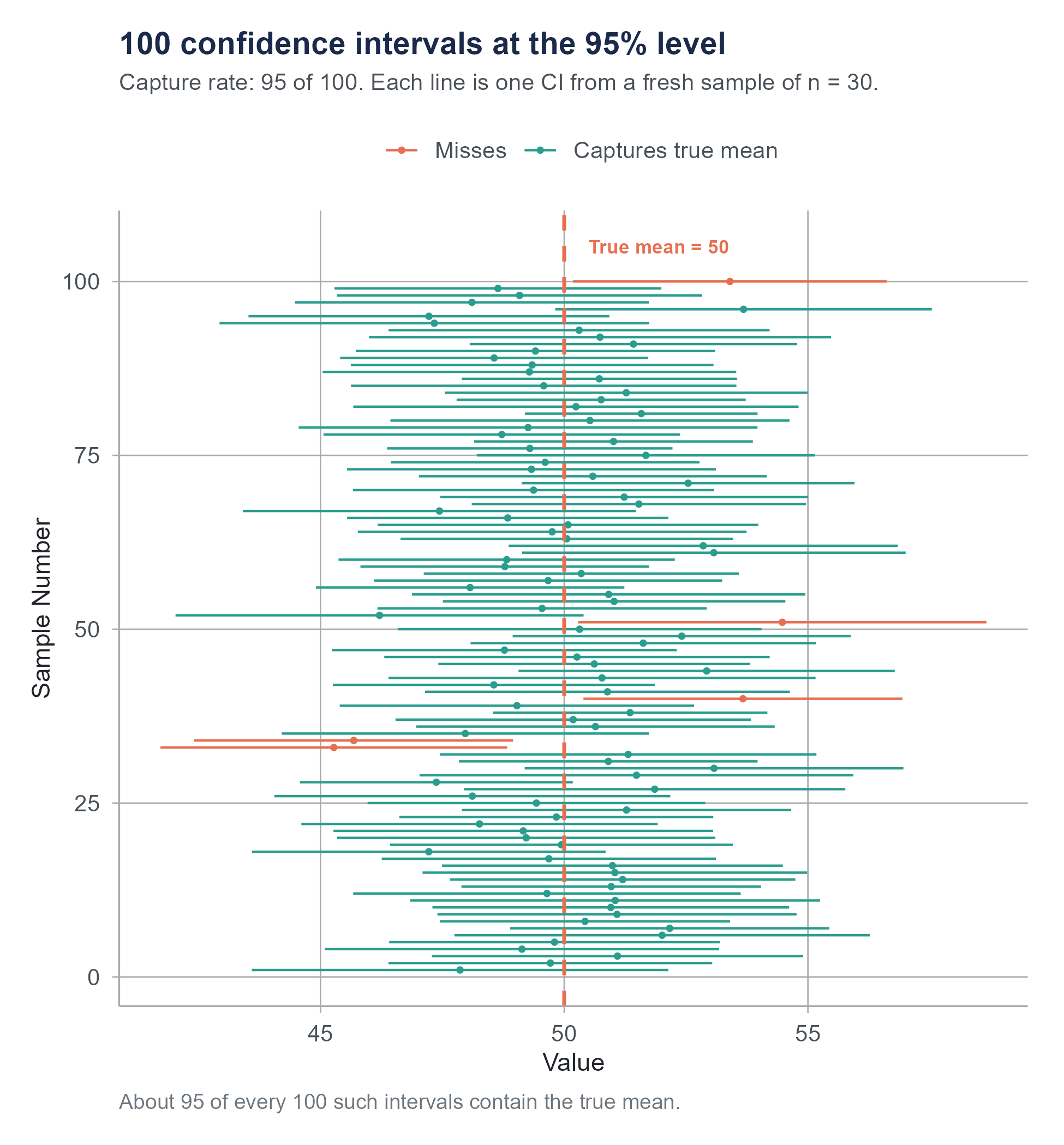
It means this: if we were to repeat the entire sampling process many, many times, each time drawing a new random sample of 36 patients and computing a new 95% confidence interval, then about 95% of those intervals would contain the true population mean. And about 5% would miss it.

The confidence level describes the long-run reliability of the method, not the probability of any single interval being correct. It is a statement about the procedure, not about the result.

Think of it like a factory that manufactures fishing nets. The factory claims that 95% of its nets are strong enough to hold a 20-pound fish. You buy one net. Does your specific net have a 95% chance of holding? No. Your net is either strong enough or it is not. The 95% describes the production process. Out of every 100 nets the factory makes, about 95 of them will hold and about 5 will tear. You just do not know which kind you got.

Similarly, your specific confidence interval either caught the true parameter or it did not. The “95%” tells you that the method you used to build it is one that catches the true parameter 95% of the time across many uses.

7.6.1 Why This Distinction Matters

You might think this is philosophical hairsplitting. It is not. The distinction has practical consequences.

If you believe “95% probability the parameter is in my interval,” you might treat the interval as near-certainty and make bold decisions based on it. If you understand that the interval was produced by a method with a 5% miss rate, you stay appropriately humble. One in twenty intervals produced this way misses the mark. And you cannot tell by looking at the interval whether this is one of the nineteen good ones or the one bad one.

This understanding also helps explain why different researchers studying the same question can get different confidence intervals, and why they sometimes disagree. Two polling firms survey the same electorate and get different results. Neither one is wrong. Both are working with different samples, and their intervals reflect the variability inherent in sampling. Sometimes one interval will contain the true value and the other will not, and that is exactly what a 5% miss rate predicts.

Try It Online

Open the Confidence Interval Simulator on the companion website. Set the true population mean and generate 100 confidence intervals from random samples. Watch how most intervals capture the true mean, but a few miss. Change the confidence level from 95% to 90% to 99% and see how the miss rate changes. This is the single best way to internalize what confidence level means. Do not skip this one.

7.6.2 Common Misinterpretations (and Corrections)

Let us go through the most frequent ways people get confidence intervals wrong.

Wrong: “There is a 95% chance that the true mean is between 42.2 and 52.2.” Correct: “We are 95% confident that the true mean is between 42.2 and 52.2, meaning the method we used produces intervals that capture the true mean 95% of the time.”

Wrong: “95% of the data falls between 42.2 and 52.2.” Correct: The confidence interval is about the population mean, not about individual data points. Individual ER wait times could range from 5 minutes to 3 hours. The interval estimates where the average is, not where individual values are.

Wrong: “If we repeat the study, there is a 95% chance the new sample mean will fall in this interval.” Correct: A new sample mean will have its own sampling variability and could land anywhere. The interval estimates the population parameter, not future sample statistics.

Wrong: “This interval proves the population mean is not 40.” Correct: If 40 is outside the interval, the data provides evidence against 40 as the population mean. But a confidence interval does not “prove” anything. A different sample might yield a different interval that does include 40.

Wrong: “The confidence interval is so narrow that we basically know the exact value.” Correct: A narrow interval means the estimate is precise, but precision is not the same as accuracy. If the sampling method was biased (for instance, if the ER only tracked wait times for patients who checked in electronically, missing those who arrived by ambulance), the interval could be precisely wrong. It would precisely estimate the wrong quantity. Narrow intervals are nice, but they cannot fix problems that originate before the math begins.

These misinterpretations extend well beyond the classroom. They appear in published research, in news coverage, and in corporate boardrooms. A 2014 study by Hoekstra and colleagues surveyed researchers and students across multiple disciplines and found that a majority could not correctly identify the meaning of a 95% confidence interval when given multiple-choice options. The people producing the intervals often misunderstand them just as badly as the people reading them. If that feels discouraging, consider the upside: understanding this one concept puts you ahead of a large portion of practicing professionals.

7.7 What Makes Confidence Intervals Wider or Narrower

Understanding what drives the width of a confidence interval gives you practical control over the precision of your estimates. Three factors determine the width, and each one works in an intuitive way.

7.7.1 Confidence Level

Wanting to be more confident means casting a wider net. A 99% confidence interval is wider than a 95% interval, which is wider than a 90% interval. The critical value ($t^*$ or $z^*$) increases as the confidence level goes up.

For a z-based interval, $z^*$ at 90% is 1.645, at 95% is 1.96, and at 99% is 2.576. Moving from 95% to 99% confidence increases the critical value by about 31%, which stretches the interval substantially. You are trading precision for confidence. Most of the time, 95% represents a reasonable compromise, which is why it has become the default in most fields.

7.7.2 Sample Size

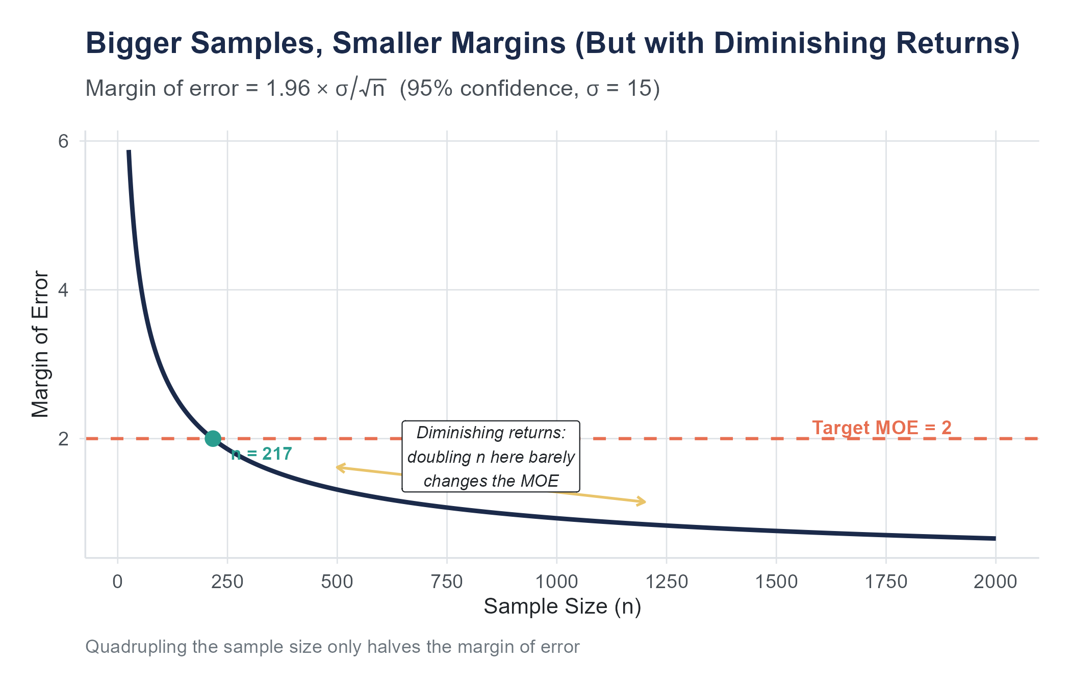
Larger samples produce narrower intervals. The standard error has $\sqrt{n}$ in the denominator, so as $n$ grows, the standard error shrinks, and the margin of error follows.

But notice the square root. Doubling your sample size does not cut the margin of error in half. It reduces it by a factor of $\sqrt{2} \approx 1.41$, which means about a 29% reduction. To halve the margin of error, you need four times the sample size. To cut it to one-third, you need nine times the data. This is the law of diminishing returns in sampling. The first hundred observations buy you a lot of precision. Going from 10,000 to 10,100 buys you almost nothing.

Figure 7.2: Margin of error plotted against sample size, showing the characteristic curve of diminishing returns. The margin of error drops steeply at first but flattens out for larger samples, illustrating why quadrupling the sample size only halves the margin of error.

7.7.3 Variability in the Data

More variability in the population, captured by $s$ in the formula, leads to wider confidence intervals. This makes sense. If everyone in the population is similar, a small sample tells you a lot. If there is enormous variation, you need more data to pin down the center.

You have limited control over population variability. It is a property of the thing you are studying. Wait times in an emergency department are inherently more variable than, say, the weight of machine-produced bolts. But you can sometimes reduce variability by narrowing your population (studying wait times for a specific type of visit, for example) or by using more precise measurement instruments.

Here is a concrete way to feel the interplay of these three factors. Imagine you are trying to estimate the average household income in a medium-sized city. You survey 100 households and compute a 95% confidence interval. It runs from $52,000 to $68,000, a range of $16,000. You want the range to be narrower. You have three options, and they are not equally practical.

Option one: lower the confidence level from 95% to 90%. This narrows the interval, but now you are less confident it contains the true mean. You have traded safety for precision.

Option two: increase the sample size. If you survey 400 households instead of 100, you cut the standard error roughly in half, and the interval shrinks to maybe a $8,000 range. This costs money and time, but it gives you both precision and the same level of confidence.

Option three: reduce variability. Instead of surveying all households, you could restrict your study to, say, households with two working adults. This group is likely more homogeneous in income, so $s$ drops and the interval narrows. But now your interval estimates the mean income only for that subgroup, not for all households. You have gained precision by asking a narrower question.

Each option involves a tradeoff. Statistics is, at its heart, the art of managing these tradeoffs wisely.

7.7.4 A Summary Table

To make the interval…	You can…
Narrower (more precise)	Increase sample size
Narrower (more precise)	Accept a lower confidence level
Narrower (more precise)	Reduce variability (if possible)
Wider (more conservative)	Decrease sample size
Wider (more conservative)	Demand a higher confidence level
Wider (more conservative)	Study a more variable population

Try It Online

Return to the Sampling Explorer you first met in Chapter 2. Its confidence-interval and sample-size sections put a slider on each of the three knobs you have just read about — confidence level, sample size, and variability — and show the resulting margin of error live. Hold the population shape and the confidence level fixed, then drag the sample-size slider from 25 up to 400 and watch the margin of error fall, but at a slowing rate.

7.8 Choosing the Right Sample Size

In many practical situations, you know how precise you want your estimate to be before you collect the data. A pharmaceutical company needs to estimate a drug’s effect within a certain margin. A polling firm promises a margin of error of plus or minus 3 percentage points. A quality engineer needs to estimate the average defect rate within 0.5 percentage points.

In all these cases, the question is the same. How large a sample do I need to achieve a desired margin of error?

7.8.1 Sample Size for a Mean

Starting from the confidence interval formula, the margin of error for a mean is

\[ME = t^* \times \frac{s}{\sqrt{n}}\]

If we solve for $n$, we get

\[n = \left(\frac{t^* \times s}{ME}\right)^2\]

In practice, at the planning stage we usually do not know $s$ yet (we have not collected the data), and $t^*$ depends on $n$ through the degrees of freedom, creating a circular problem. The common approach is to use $z^*$ instead of $t^*$ for planning purposes and to estimate $s$ from a pilot study, prior research, or an educated guess. The planning formula becomes

\[n = \left(\frac{z^* \times \sigma}{ME}\right)^2\]

where $\sigma$ is your best prior estimate of the population standard deviation.

For example, suppose you want to estimate the average monthly grocery spending for families in a city within $\pm\$25$ at the 95% confidence level. From previous surveys, you believe the standard deviation is about $\$180$. Then

\[n = \left(\frac{1.96 \times 180}{25}\right)^2 = \left(\frac{352.8}{25}\right)^2 = (14.112)^2 = 199.1\]

Round up to $n = 200$. You need a sample of about 200 families. Always round up when computing required sample sizes, because rounding down gives you a margin of error slightly larger than what you wanted.

7.8.2 Sample Size for a Proportion

The margin of error for a proportion is

\[ME = z^* \times \sqrt{\frac{p(1-p)}{n}}\]

Solving for $n$ gives

\[n = \frac{(z^*)^2 \times p(1-p)}{ME^2}\]

Here we need a prior estimate of $p$, the population proportion. If you have no idea what $p$ is, the conservative approach is to use $p = 0.5$, because $p(1-p)$ is maximized at 0.5 and the resulting sample size will be the largest (most conservative) it could be. You will never underestimate the required sample size this way.

For instance, a polling organization wants a margin of error of $\pm 3$ percentage points (0.03) at the 95% confidence level. Using $p = 0.5$,

\[n = \frac{(1.96)^2 \times 0.5 \times 0.5}{(0.03)^2} = \frac{3.8416 \times 0.25}{0.0009} = \frac{0.9604}{0.0009} = 1067.1\]

Round up to 1,068. This is why national polls typically survey around 1,000 to 1,200 people. That sample size gives a margin of error in the neighborhood of $\pm 3$ percentage points at the 95% confidence level, regardless of the size of the population. A poll of 1,100 Americans has the same margin of error whether the country has 300 million people or 3 billion. The precision depends on the sample size, not on what fraction of the population you sample.

That last point surprises most people. It seems like a sample of 1,100 out of 330 million could not possibly tell you anything useful. But the mathematics says otherwise. The key is that each sampled person provides an independent piece of information about the population. As long as the sample is random, 1,100 independent data points constrain the population proportion to within about 3 percentage points with 95% confidence.

7.9 Connecting Back to the Polls

Now you have the tools to understand what happened in those election nights.

When a pre-election poll reports “Candidate A: 48%, Candidate B: 45%, margin of error $\pm 3.5$ points,” here is what it is actually saying. The 95% confidence interval for Candidate A’s support is roughly 44.5% to 51.5%. The interval for Candidate B is roughly 41.5% to 48.5%. Those intervals overlap considerably. The poll is consistent with Candidate A winning comfortably, with Candidate B winning, or with a near tie.

But the headline says “Candidate A Leads.” And readers think the race is decided.

The 2016 and 2020 elections illustrated this gap between what the data said and what people heard. In 2016, many state-level polls were within their margins of error, but those margins of error were wide enough to include a Trump win. People who understood confidence intervals were less surprised. Nate Silver, who gave Trump a 29% chance, was widely mocked before the election for being too generous to Trump, and widely cited afterward for being the forecaster who got it “least wrong.” His model was not magic. It was just taking the uncertainty in the polls seriously.

In 2020, the polling errors were larger, pointing to real methodological challenges with reaching certain segments of the population. Even so, most results fell within the 95% confidence bands when you account for the full range of uncertainty including potential correlated errors across states. The lesson is not that polls are useless. The lesson is that the margin of error is not a decoration. It is the most informative part of the result.

There is a useful habit you can develop the next time you see a poll in the news. Before looking at who is “ahead,” look at the margin of error. Subtract the margin of error from the leading candidate’s number and add it to the trailing candidate’s number. If the result flips the lead, the poll is telling you the race is too close to call. If the lead survives even the worst-case interpretation, you have something more meaningful. This takes about five seconds and it transforms you from a passive consumer of poll headlines into someone who actually reads the data. Most people never bother. You should.

7.10 Ethics of Sample Size

We have talked about sample size as a matter of precision. But it is also a matter of ethics.

Consider a medical study designed to test whether a new drug reduces blood pressure. If the researchers enroll too few patients, the confidence interval for the drug’s effect will be wide. So wide that even if the drug works, the study will not be able to detect the effect. The confidence interval will include both “the drug works” and “the drug does not work,” and the study will be inconclusive.

This is more than a statistical failure. It is an ethical one.

Ethics Moment

An underpowered study, one with a sample too small to detect the effect it is looking for, wastes resources and can cause real harm. Patients in the study were exposed to the risks of an experimental treatment without any chance of producing useful knowledge. Grant funding was consumed without returning answers. And the inconclusive results might discourage future research on a treatment that actually works, depriving future patients of a beneficial therapy.

Research ethics boards require investigators to justify their sample sizes before a study begins. A sample size calculation, based on the desired margin of error and the expected effect size, is more than a statistical formality. It is an ethical obligation. Running a study you know is too small to answer the question is a misuse of participants’ trust, their time, and in many cases their bodies.

This principle extends beyond medicine. Business A/B tests with samples too small to detect meaningful differences waste company resources and delay decisions. Surveys with inadequate sample sizes in certain demographic groups can render those groups statistically invisible, leading to policies and products that do not account for their needs. Whenever you plan a study, asking “Is my sample large enough?” is more than a technical question. It is a question about whether you are being responsible with the resources and the people involved.

7.11 Putting It All Together

Let us revisit the structure of this chapter by walking through one more complete example that ties together all the pieces.

A chain of coffee shops wants to estimate the average amount customers spend per visit. They randomly sample 50 transactions from across their locations and record the amount spent. The sample mean is $\bar{x} = \$6.85$ and the sample standard deviation is $s = \$2.40$.

Constructing a 95% confidence interval for the mean.

Point estimate. $\bar{x} = 6.85$.
Degrees of freedom. $df = 50 - 1 = 49$.
Critical value. $t^*$ for 95% confidence with 49 degrees of freedom is approximately 2.010.
Standard error. $SE = \frac{2.40}{\sqrt{50}} = \frac{2.40}{7.071} = 0.3394$.
Margin of error. $ME = 2.010 \times 0.3394 = 0.682$.
Confidence interval. $6.85 \pm 0.682 = (6.17, 7.53)$.

Interpretation. We are 95% confident that the average amount spent per visit across all customers at this coffee shop chain is between $6.17 and $7.53. This means that if we were to repeat this process many times, drawing new random samples of 50 transactions each time and computing a confidence interval, about 95% of those intervals would contain the true average spending amount.

What if the chain wanted a narrower interval? They could increase the sample size. If they sampled 200 transactions instead of 50, the standard error would drop to $\frac{2.40}{\sqrt{200}} = 0.1697$, and the margin of error would shrink to about $0.34$, giving an interval roughly half as wide.

What if they wanted 99% confidence instead of 95%? The critical value would increase to about 2.680, and the margin of error would grow to $2.680 \times 0.3394 = 0.910$, giving a wider interval of $(5.94, 7.76)$. More confidence, less precision.

Now suppose the company wants to plan a future, larger study. They want the margin of error to be no more than $\pm\$0.50$ at the 95% confidence level. Using the planning formula with $\sigma \approx 2.40$,

\[n = \left(\frac{1.96 \times 2.40}{0.50}\right)^2 = \left(\frac{4.704}{0.50}\right)^2 = (9.408)^2 = 88.5\]

They need at least 89 transactions. This is manageable. If they wanted $\pm\$0.25$, they would need

\[n = \left(\frac{1.96 \times 2.40}{0.25}\right)^2 = (18.816)^2 = 354.0\]

At least 354 transactions. Notice how halving the desired margin of error nearly quadrupled the required sample.

Try It Online

Two apps work well together as you finish this chapter.

The Confidence Interval Simulator is the place to feel what “95% confidence” actually means — generate hundreds of intervals and record what fraction capture the true parameter at the 90%, 95%, and 99% levels.
The Sampling Explorer’s sample-size calculator is the place to plan a study before you collect data — pick the kind of estimate, the desired margin of error, and the confidence level, and the app tells you the required $n$ that the formulas in this section produce.

7.12 A Few Final Cautions

Confidence intervals are only as good as your data. A confidence interval based on a biased sample is a precise estimate of the wrong thing. If the coffee shop only sampled transactions from its busiest location on Saturday mornings, the interval would be precise but misleading. Random sampling matters.

Confidence intervals assume the conditions are met. If the data is not independent, or if the sample is too small and the distribution is heavily skewed, the interval’s stated confidence level may not match its actual reliability. Always check conditions.

A narrow confidence interval does not mean the estimate is correct. It means the estimate is precise. Precision and accuracy are different things. You can be precisely wrong if your sampling method is biased or your measurement is flawed. A confidence interval quantifies sampling variability. It does not account for other sources of error, like measurement bias, nonresponse bias, or data processing mistakes.

Do not confuse statistical confidence with practical importance. A 95% confidence interval of (0.01, 0.03) for the difference in click-through rates between two website designs is very precise and estimates the true difference to fall between 1 and 3 percentage points. Whether that difference matters for your business depends on context, not on the confidence level.

AI Reality Check

Ask an AI tool to analyze a dataset and it will almost always give you a point estimate. “The average is 47.3.” Sometimes it will even give you a confidence interval. But watch what it does with that interval.

AI tools frequently report confidence intervals without checking whether the conditions for constructing them are met. They may compute a confidence interval for a mean from a sample of 12 observations drawn from a heavily skewed distribution, where the t-interval is unreliable. They may construct a confidence interval for a proportion when the sample size is too small for the normal approximation (the success-failure condition fails). They may even generate a confidence interval from a convenience sample and present it as if it quantifies uncertainty about the population, when in fact the biggest source of uncertainty is the non-random sampling, which no formula can fix.

Perhaps more subtly, AI tools tend to present confidence intervals as final answers rather than as starting points for interpretation. A confidence interval is not a conclusion. It is a tool for thinking about uncertainty. Whether the interval is wide enough to change your decision, whether it includes practically meaningful values, whether the sample it is based on actually represents the population you care about, these are judgment calls that require context the AI does not have. Use AI to compute the interval. Use your own thinking to decide what it means.

7.13 Looking Ahead

This chapter introduced the first formal tool of statistical inference: the confidence interval. You now know how to move from a single sample statistic to a range of plausible values for a population parameter, and you understand what “95% confident” actually means (and what it does not mean). But confidence intervals answer only one kind of question: “What are the plausible values?” They do not answer “Is there evidence against a specific claim?” That is the subject of hypothesis testing. In the next chapter, we will learn to formalize the question “Could this result have happened by chance?” and develop a rigorous framework for deciding when the data provides evidence against a null hypothesis. The logic of hypothesis testing will draw directly on the sampling distributions and standard errors we have built up over the past two chapters.

7.14 Further Reading and References

The following works are cited in this chapter or provide valuable additional context for the ideas covered here.

On the interpretation of confidence intervals: Hoekstra, R., Morey, R. D., Rouder, J. N., & Wagenmakers, E.-J. (2014). Robust misinterpretation of confidence intervals. Psychonomic Bulletin & Review, 21(5), 1157–1164. (A study documenting how frequently researchers misinterpret confidence intervals, even among those with statistical training.)

On polling methodology and election forecasting: Silver, N. (2012). The signal and the noise: Why so many predictions fail — but some don’t. Penguin. (An accessible treatment of forecasting, uncertainty, and the role of probability in interpreting polls, written by the founder of FiveThirtyEight.)

Kennedy, C., Blumenthal, M., Clement, S., Clinton, J. D., Durand, C., Franklin, C., McGeeney, K., Miringoff, L., Olson, K., Rivers, D., Saad, L., Witt, G. E., & Wlezien, C. (2018). An evaluation of the 2016 election polls in the United States. Public Opinion Quarterly, 82(1), 1–33. (The American Association for Public Opinion Research’s official post-mortem on what went wrong with the 2016 polls and what it means for margin-of-error reporting.)

On sample size planning and ethical dimensions: Lenth, R. V. (2001). Some practical guidelines for effective sample size determination. The American Statistician, 55(3), 187–193. (A concise discussion of the practical and ethical considerations involved in choosing a sample size, emphasizing that underpowered studies waste resources and participants’ contributions.)

For further reading on confidence intervals: Cumming, G. (2012). Understanding the new statistics: Effect sizes, confidence intervals, and meta-analysis. Routledge. (A clear, visual approach to confidence intervals and effect sizes that argues for moving beyond p-values toward interval estimation as the primary tool of inference.)

7.15 Key Terms

Point estimate: A single value computed from sample data that serves as the best guess for a population parameter. Examples include the sample mean $\bar{x}$ and the sample proportion $\hat{p}$.
Interval estimate: A range of plausible values for a population parameter, constructed from sample data. A confidence interval is the most common type.
Confidence interval: A range of plausible values for a population parameter, constructed from sample data as (point estimate $\pm$ margin of error). A 95% confidence interval means that 95% of intervals constructed this way would contain the true parameter.
Margin of error: The amount added to and subtracted from the point estimate to form the confidence interval. Equals the critical value times the standard error.
Standard error: The estimated standard deviation of a sampling distribution. Measures how much a sample statistic would vary across repeated samples. For a mean, $SE = \frac{s}{\sqrt{n}}$. For a proportion, $SE = \sqrt{\frac{\hat{p}(1-\hat{p})}{n}}$.
Critical value: The multiplier ($t^*$ or $z^*$) that determines how many standard errors wide the confidence interval extends. Depends on the desired confidence level and, for the t-distribution, the degrees of freedom.
t-distribution: A family of bell-shaped distributions, indexed by degrees of freedom, used for inference about means when the population standard deviation is unknown. Has heavier tails than the normal distribution, especially at low degrees of freedom.
Degrees of freedom: A parameter of the t-distribution equal to $n - 1$ for a single-sample mean. Reflects the amount of independent information available for estimating variability.
Confidence level: The long-run proportion of confidence intervals that would contain the true parameter if the sampling process were repeated many times. Common levels are 90%, 95%, and 99%.
Sample size determination: The process of calculating how large a sample is needed to achieve a desired margin of error at a given confidence level.
Underpowered study: A study with a sample too small to detect the effect of interest with reasonable confidence, raising both statistical and ethical concerns.

7.16 Exercises

7.16.1 Check Your Understanding

Explain in your own words why a point estimate alone is insufficient for drawing conclusions about a population parameter.
Write out the general form of a confidence interval. Identify each component and explain what it contributes.
A 95% confidence interval for the average commute time in a city is (22.4, 28.6) minutes. A student says, “There is a 95% probability that the true average commute time is between 22.4 and 28.6 minutes.” What is wrong with this interpretation? Provide a correct one.
Explain why we use the t-distribution rather than the z-distribution when constructing a confidence interval for a mean. Under what circumstances does the choice between t and z matter most?
What are degrees of freedom, and why does a confidence interval for a single mean use $n - 1$ degrees of freedom?
List three factors that affect the width of a confidence interval. For each one, state whether increasing it makes the interval wider or narrower, and explain why.
A researcher constructs a 90% confidence interval and a 99% confidence interval from the same data. Which interval is wider? Why?
A poll reports that 52% of voters support a ballot measure, with a margin of error of $\pm 4$ percentage points. A news anchor says, “The measure has majority support.” Is this claim justified by the poll? Explain.
Suppose you double the sample size while everything else stays the same. By what factor does the margin of error change? Show your reasoning.
Explain what the success-failure condition is for a confidence interval for a proportion, and why it is necessary.

7.16.2 Apply It

A random sample of 25 college students reports the following weekly study hours. The sample mean is $\bar{x} = 14.3$ hours and the sample standard deviation is $s = 4.1$ hours. Construct a 95% confidence interval for the mean weekly study hours of all college students at this university. Show all steps and interpret the result.
In a sample of 800 adults, 328 report that they have visited a dentist in the past six months. Construct a 99% confidence interval for the true proportion of adults who have visited a dentist in the past six months. Verify that the conditions for the interval are met.
A food safety inspector takes a random sample of 40 chicken breast packages from a processing plant and measures the weight of each. The sample yields $\bar{x} = 1.02$ pounds and $s = 0.08$ pounds. The packages are labeled as containing 1.00 pound. Construct a 95% confidence interval for the mean weight. Based on your interval, does the evidence suggest the packages are accurately labeled?
A technology company surveys 1,500 of its users and finds that 63% are satisfied with the latest software update. Construct a 95% confidence interval for the true proportion of satisfied users. If the company’s goal was to achieve at least 60% satisfaction, what can you conclude?
A researcher wants to estimate the average daily screen time for teenagers in the United States within $\pm 15$ minutes at the 95% confidence level. Previous studies suggest the standard deviation of daily screen time is about 90 minutes. How large a sample does the researcher need?
A political campaign wants to estimate the proportion of voters who recognize the candidate’s name, with a margin of error of no more than $\pm 2$ percentage points at the 95% confidence level. The campaign has no prior estimate of name recognition. What sample size is needed?
A hospital collects data on the recovery time (in days) for patients after a certain surgery. A sample of 18 patients has a mean recovery time of $\bar{x} = 5.8$ days and a standard deviation of $s = 1.9$ days. Construct a 90% confidence interval for the mean recovery time. What additional assumption should you check given the relatively small sample size?
Two polling organizations survey the same electorate. Poll A, based on $n = 1,000$, reports 48% support for a candidate with a margin of error of $\pm 3.1\%$. Poll B, based on $n = 2,500$, reports 51% support with a margin of error of $\pm 2.0\%$. The two confidence intervals overlap. Are the polls contradicting each other? Explain.
A quality control manager samples 60 light bulbs and measures their lifetimes. The sample mean is $\bar{x} = 1,020$ hours and $s = 85$ hours. Construct 90%, 95%, and 99% confidence intervals for the true mean lifetime. Present all three intervals and comment on how the width changes as the confidence level increases.
A nonprofit organization wants to estimate the proportion of residents in a neighborhood who would use a proposed community garden. They conduct a pilot survey of 50 residents and find that 34 would use the garden. (a) Construct a 95% confidence interval based on the pilot survey. (b) The organization considers this interval too wide and wants a margin of error of $\pm 5$ percentage points. Using the pilot estimate as a guide, how many residents should they survey?

The following three exercises use the polling-data.csv dataset available on the companion website. This is real polling data drawn from FiveThirtyEight’s pollster ratings dataset. The dataset contains 50 observations with variables including poll_id, pollster (polling organization), date, sample_size, candidate_a_pct, candidate_b_pct, margin_of_error, and confidence_level.

Using the polling-data.csv dataset, select any single poll and verify its reported margin of error. Using the reported candidate_a_pct as your sample proportion $\hat{p}$ and the poll’s sample_size as $n$, compute the margin of error for a 95% confidence interval using the formula $ME = z^* \sqrt{\hat{p}(1-\hat{p})/n}$. How close is your calculated margin of error to the value reported in the margin_of_error column? What might explain any difference?
Compute the mean and standard deviation of candidate_a_pct across all 50 polls. Construct a 95% confidence interval for the mean of candidate_a_pct across polls. Then identify how many of the 50 individual polls have a candidate_a_pct value outside this interval. Is the observed count consistent with what you would expect? Now create a scatter plot of sample_size (horizontal axis) versus margin_of_error (vertical axis). Describe the pattern. Does the relationship match what the formula $ME \propto 1/\sqrt{n}$ predicts?
Sort the polls by sample_size. Compare the five polls with the largest sample sizes to the five polls with the smallest sample sizes. For each group, compute the mean and standard deviation of candidate_a_pct. Which group shows more variability in its estimates? Construct a 95% confidence interval for the mean of candidate_a_pct within each group. Which group’s interval is narrower? Explain why, using the concept of the sampling distribution.

7.16.3 Think Deeper

A news article reports, “A new study finds that the average American spends 2.5 hours per day on social media, with a 95% confidence interval of (2.3, 2.7) hours.” The study was conducted using an online survey promoted through social media platforms. Discuss at least two reasons why the confidence interval, despite being correctly calculated, might not give a trustworthy estimate of the true average for all Americans. What types of error does a confidence interval account for, and what types does it not?
During the COVID-19 pandemic, early estimates of the virus’s infection fatality rate varied widely across studies, partly because different studies had very different sample sizes and sampling methods. Some early estimates from small samples had very wide confidence intervals. How should policymakers use confidence intervals when making urgent decisions with limited data? Is it better to act on a point estimate from a small study or to wait for more precise data? What are the risks of each approach?
Consider two studies investigating the same question: whether a job training program increases employment rates among participants. Study A enrolls 40 participants and finds an employment rate of 68%, with a 95% confidence interval of (53%, 83%). Study B enrolls 500 participants and finds an employment rate of 61%, with a 95% confidence interval of (57%, 65%). Study A’s point estimate is higher, but Study B’s interval is much narrower. Which study provides more useful evidence for deciding whether to expand the program? What does each study tell you that the other does not? How does sample size relate to the ethical obligation to produce actionable knowledge?
A pharmaceutical company runs a clinical trial with 5,000 participants and finds that its new drug lowers cholesterol by an average of 3 mg/dL, with a 95% confidence interval of (2.1, 3.9) mg/dL. The interval does not include zero, so the effect is statistically distinguishable from no effect. However, physicians consider a reduction of less than 10 mg/dL to be clinically meaningless. Discuss the difference between statistical confidence and practical importance. Should this drug be brought to market based on this evidence? What additional information would you want?
Return to the opening story about election polling. Some commentators have suggested that polls should stop reporting a single topline number and margin of error, and instead only report the full confidence interval or a probability distribution of possible outcomes. What would be gained and what would be lost by this approach? Consider the needs of different audiences, including voters, journalists, campaign strategists, and election administrators. Is there a tension between statistical accuracy and public communication?