5 Probability: Thinking About Chance
5.1 The Test Said Yes
In the spring of 2020, as COVID-19 spread across the world, a question consumed millions of people. If my test comes back positive, does that mean I have the virus?
The answer, it turned out, was “not necessarily.” And the reason is a foundational idea in statistics.
Here is a simplified but realistic scenario from the early months of the pandemic. Suppose you lived in a community where about 1% of the population was actually infected at a given time. Suppose you took a rapid antigen test with the following performance characteristics, which were roughly in line with many tests on the market. If you truly had the virus, the test correctly came back positive about 90% of the time. If you did not have the virus, the test correctly came back negative about 95% of the time.
Now suppose you tested positive. How worried should you have been?
Most people, including many physicians, would have said something like “the test is 90% accurate, so there is about a 90% chance you are infected.” That answer is wrong. It is not a little wrong. It is sharply wrong.
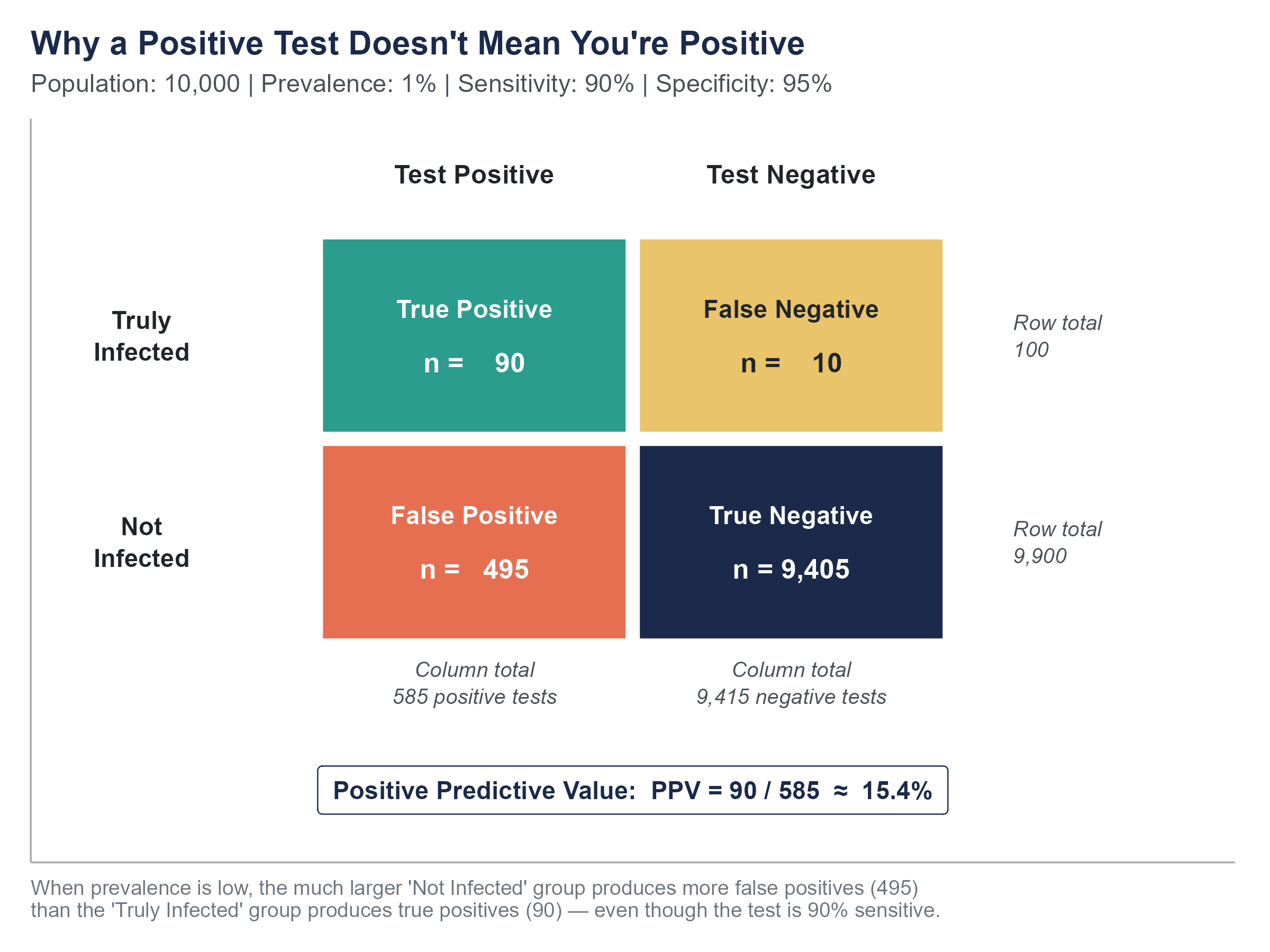
Let’s work through the math with a concrete group. Imagine 10,000 people from this community get tested. Since 1% are truly infected, that gives us 100 people with the virus and 9,900 without it. Of the 100 infected people, 90% test positive, so 90 get a correct positive result. Of the 9,900 uninfected people, 5% get a false positive, so 495 people who do not have the virus are told they do.
Add up all the positive tests. That’s \(90 + 495 = 585\) positive results. Of those 585 people staring at a positive test, only 90 actually have the virus. That means the probability that you truly have COVID given a positive test is \(90 / 585 \approx 15.4\%\).
Read that again. A positive result on this test, in this community, meant about a 15% chance you were actually infected. More than 8 out of 10 people with positive results were false alarms.
This is not a failure of the test. The test performed exactly as advertised. This is a consequence of a low base rate, the proportion of people in the population who actually had the condition. When the base rate is low, even a good test produces more false positives than true positives, simply because the “healthy” group is so much larger than the “sick” group.
Understanding this requires understanding probability, and specifically a result called Bayes’ theorem. That is the destination of this chapter. Along the way, we will build the fundamental rules of probability from the ground up, because Bayes’ theorem does not come out of nowhere. It is a logical consequence of how probabilities combine.
During the pandemic, this misunderstanding had real consequences. People who tested positive entered mandatory quarantine, cancelled surgeries, pulled children from school, and isolated from dying relatives, sometimes on the basis of a result that was more likely to be wrong than right. Meanwhile, people who tested negative felt invincible and went about their lives, even though some of them were actually infected. The errors ran in both directions, and the human cost was substantial.
None of this means testing was useless. It means that interpreting a test result requires more information than the result itself. You need to know the base rate, the test’s sensitivity, and the test’s specificity. And you need to know how to combine them. That is what this chapter teaches.
Before you read another word, open the Base Rate Lab on the companion website and go to the Natural Frequencies tab. It shows the 10,000-person tree from the COVID story, live. Drag the prevalence slider from 1% down toward 0.1% and watch the “true positive” and “false positive” piles at the bottom of the tree. The positive predictive value (the chance you’re really infected given a positive test) collapses toward zero even though the test itself hasn’t changed at all. That collapse is the whole lesson of this chapter, and it is much easier to feel than to memorize.
5.2 What Probability Means
Before we calculate anything, we need to agree on what probability is. This turns out to be less obvious than it sounds, and professional statisticians have argued about it for more than a century.
There are three main interpretations.
The classical interpretation defines probability as the number of favorable outcomes divided by the total number of equally likely outcomes. The probability of rolling a 3 on a fair die is \(1/6\) because there are six equally likely faces and one of them is a 3. This works well for dice, cards, and coins, but it struggles when outcomes are not equally likely, or when you cannot enumerate them.
The frequentist interpretation defines probability as the long-run relative frequency of an event. If you flip a coin thousands of times, the proportion of heads will settle near 0.5. The probability of heads is that long-run proportion. This interpretation is practical and intuitive for repeatable events, but it gets awkward when you want to talk about the probability of a one-time event, like the probability that a specific candidate wins an election.
The Bayesian (or subjectivist) interpretation defines probability as a degree of belief in a proposition, conditional on the evidence available. A doctor estimating a 10% chance that a patient’s tumor is malignant before any biopsy, or an election analyst pegging a 65% probability that a particular candidate wins on Tuesday, is expressing a degree of belief about a single, non-repeatable situation. This interpretation handles one-time events naturally, but it requires a framework for updating beliefs as new evidence arrives. That framework, as you might guess, is Bayes’ theorem.
For this book, we will use whichever interpretation makes sense for the problem at hand. In practice, most working statisticians move between interpretations depending on context, even if they have strong philosophical preferences. What matters for now is the mathematical machinery, which is the same regardless of interpretation.
5.2.1 The Language of Probability
An experiment (or random process) is any procedure that produces an uncertain outcome. Rolling a die, drawing a card, testing a patient, surveying a voter.
The sample space, denoted \(S\), is the set of all possible outcomes. For a single coin flip, \(S = \{H, T\}\). For rolling a die, \(S = \{1, 2, 3, 4, 5, 6\}\).
An event is any subset of the sample space. “Rolling an even number” is the event \(\{2, 4, 6\}\). “Getting heads” is the event \(\{H\}\).
The probability of an event \(A\), written \(P(A)\), is a number between 0 and 1 (inclusive) that measures how likely the event is to occur. A probability of 0 means the event cannot happen. A probability of 1 means the event is certain. Everything else falls in between.
Two basic rules anchor everything that follows.
Rule 1. For any event \(A\), \(0 \leq P(A) \leq 1\).
Rule 2. The probabilities of all outcomes in the sample space must add up to 1. Something has to happen.
5.3 Basic Probability Rules
5.3.1 The Complement Rule
The complement of an event \(A\), written \(A^c\) (read “A complement”), is the event that \(A\) does not occur. If \(A\) is “it rains today,” then \(A^c\) is “it does not rain today.”
Since either \(A\) happens or it doesn’t, and those are the only two options,
\[P(A) + P(A^c) = 1\]
which means
\[P(A^c) = 1 - P(A)\]
This is often the easiest way to compute a probability. If the probability of at least one defective item in a shipment is hard to calculate directly, it may be much simpler to calculate the probability that no items are defective and subtract from 1.
Example. A weather forecast says there is a 35% chance of snow tomorrow. What is the probability it does not snow?
\[P(\text{no snow}) = 1 - P(\text{snow}) = 1 - 0.35 = 0.65\]
Simple, but the complement rule becomes especially powerful when combined with other rules. If you want to know the probability that at least one person in a room of 30 shares your birthday, it is much easier to compute \(1 - P(\text{nobody shares your birthday})\) than to enumerate all the ways one or more people could share it. We will see more examples like this as the chapter progresses.
5.3.2 The Addition Rule
Suppose you want to know the probability that event \(A\) or event \(B\) occurs (or both). The answer depends on whether \(A\) and \(B\) can happen at the same time.
Mutually exclusive events cannot occur simultaneously. If you roll a single die, the events “roll a 2” and “roll a 5” are mutually exclusive. You cannot get both on one roll.
For mutually exclusive events, the probability of \(A\) or \(B\) is simply the sum of their individual probabilities.
\[P(A \text{ or } B) = P(A) + P(B) \quad \text{(if } A \text{ and } B \text{ are mutually exclusive)}\]
The probability of rolling a 2 or a 5 on a fair die is \(1/6 + 1/6 = 2/6 = 1/3\).
But most events in the real world are not mutually exclusive. If you draw a card from a standard deck, the events “draw a heart” and “draw a queen” can both happen, because the queen of hearts exists. If you just add \(P(\text{heart}) + P(\text{queen}) = 13/52 + 4/52 = 17/52\), you have counted the queen of hearts twice.
The general addition rule corrects for this double-counting.
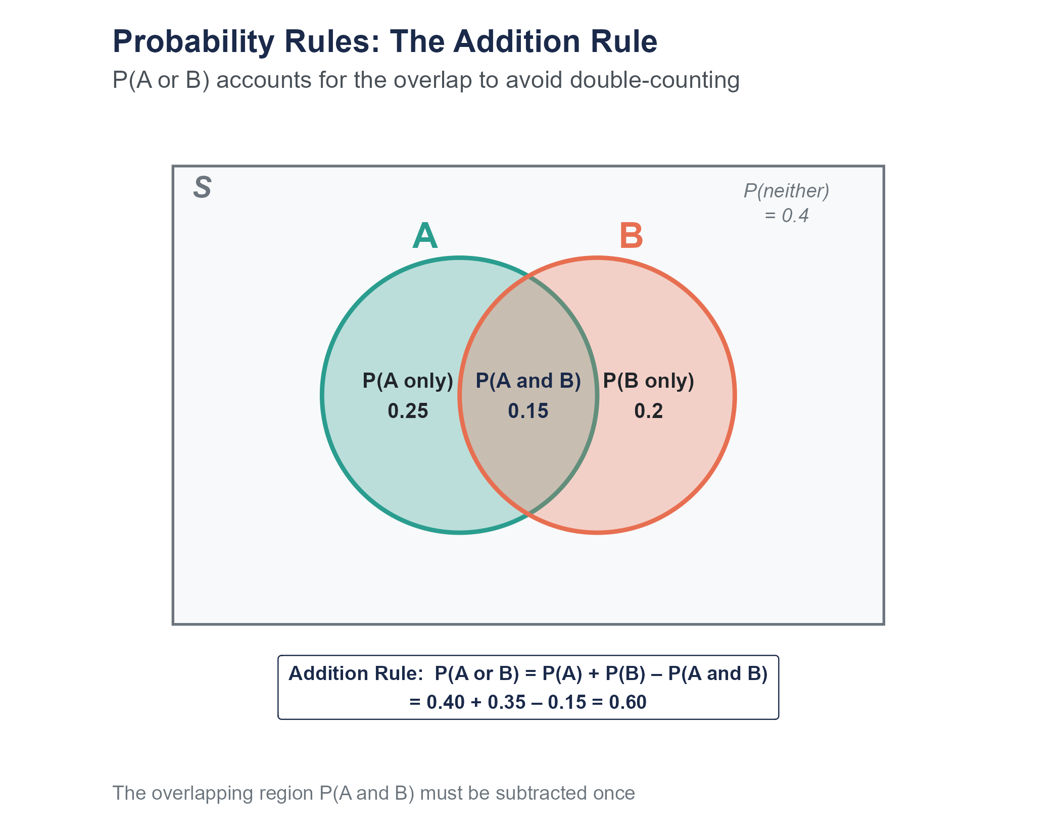
\[P(A \text{ or } B) = P(A) + P(B) - P(A \text{ and } B)\]
For our card example, \(P(\text{heart or queen}) = 13/52 + 4/52 - 1/52 = 16/52 = 4/13\).
Notice that when events are mutually exclusive, \(P(A \text{ and } B) = 0\), so the general rule simplifies to the simpler rule. The general rule always works.
The addition rule has a visual analog. If you draw a Venn diagram with two overlapping circles, the total area covered by at least one circle equals the area of circle \(A\) plus the area of circle \(B\) minus the overlap region, which you would otherwise count twice. Venn diagrams are more than decorations from middle school math. They are a useful way to keep track of which events overlap and which do not.
5.3.3 The Multiplication Rule and Independence
Now suppose you want to know the probability that event \(A\) and event \(B\) both occur. This is where the concept of independence becomes critical.
Two events are independent if the occurrence of one does not change the probability of the other. Flipping a coin and rolling a die are independent. Getting heads on the coin does not make any particular die outcome more or less likely.
For independent events, the probability that both occur is the product of their individual probabilities.
\[P(A \text{ and } B) = P(A) \times P(B) \quad \text{(if } A \text{ and } B \text{ are independent)}\]
The probability of flipping heads and rolling a 6 is \(1/2 \times 1/6 = 1/12\).
If events are not independent, we need the general multiplication rule, which uses conditional probability.
\[P(A \text{ and } B) = P(A) \times P(B \mid A)\]
We will return to this shortly, once we have defined conditional probability properly.
A word of warning. Independence is often assumed when it should not be. “What is the probability that both of my flights are delayed?” is only \(P(\text{flight 1 delayed}) \times P(\text{flight 2 delayed})\) if the two delays are independent. But if your second flight is a connection from the first, or if both fly out of the same airport during the same weather system, they are not independent, and the simple multiplication gives you the wrong answer.
Example. Suppose a manufacturing process has three independent quality checks. Each check catches a defective product with probability 0.80. What is the probability that a defective product passes all three checks undetected?
Each check independently fails to catch the defect with probability \(1 - 0.80 = 0.20\). Since the checks are independent, the probability of slipping past all three is
\[P(\text{all three miss}) = 0.20 \times 0.20 \times 0.20 = 0.008\]
Less than 1%. This is the logic behind redundant systems, from quality control to airplane safety. Each individual check might miss something, but stacking independent checks on top of each other drives the probability of total failure down rapidly.
Open the Probability Rules Sandbox on the companion website. It lets you set \(P(A)\), \(P(B)\), and \(P(A \text{ and } B)\) with sliders and watch every rule in this section update at once on a Venn diagram, a proportional unit-square view, and a tree diagram. Toggle Force independent to see the multiplication rule snap into place; toggle Force mutually exclusive to see the addition rule simplify. A small set of preset scenarios (cards, dice, weather, handedness) is included so you can check your intuition against worked examples.
5.4 Conditional Probability and Two-Way Tables
5.4.1 Conditional Probability
The conditional probability of \(A\) given \(B\), written \(P(A \mid B)\), is the probability that \(A\) occurs given that we already know \(B\) has occurred. The vertical bar \(\mid\) is read as “given.”
The formula is
\[P(A \mid B) = \frac{P(A \text{ and } B)}{P(B)}\]
provided \(P(B) > 0\). In words, to find the probability of \(A\) given \(B\), take the probability that both happen and divide by the probability of \(B\). You are essentially restricting your attention to the world where \(B\) has happened and asking how often \(A\) also happens in that restricted world.
Think of it this way. If I tell you that a randomly selected person from a room is wearing glasses, and I ask you the probability that person is over 60, you are no longer thinking about the entire room. You are mentally filtering down to only the glasses-wearers and asking what fraction of that subgroup is over 60. That mental filter is what conditional probability formalizes.
Let’s make this concrete with a two-way table.
5.4.2 Working with Two-Way Tables
Consider a hypothetical survey of 800 recent graduates from a mid-sized university about their employment status and their major category. Here are the results.
| Employed Full-Time | Employed Part-Time | Seeking Employment | Total | |
|---|---|---|---|---|
| STEM | 180 | 40 | 30 | 250 |
| Business | 150 | 45 | 25 | 220 |
| Humanities | 100 | 60 | 50 | 210 |
| Social Sciences | 80 | 25 | 15 | 120 |
| Total | 510 | 170 | 120 | 800 |
From this table, we can answer many probability questions by treating the 800 graduates as our population and computing proportions.
What is the probability that a randomly selected graduate is employed full-time?
\[P(\text{full-time}) = \frac{510}{800} = 0.6375\]
What is the probability that a randomly selected graduate is a humanities major?
\[P(\text{humanities}) = \frac{210}{800} = 0.2625\]
What is the probability that a graduate is both a STEM major and employed full-time?
\[P(\text{STEM and full-time}) = \frac{180}{800} = 0.225\]
Now for conditional probability.
Given that a graduate is a STEM major, what is the probability they are employed full-time?
We restrict our attention to the 250 STEM majors and ask how many of them are employed full-time.
\[P(\text{full-time} \mid \text{STEM}) = \frac{180}{250} = 0.72\]
Given that a graduate is employed full-time, what is the probability they are a STEM major?
Now we restrict our attention to the 510 full-time employed graduates.
\[P(\text{STEM} \mid \text{full-time}) = \frac{180}{510} \approx 0.353\]
Notice something important. \(P(\text{full-time} \mid \text{STEM}) = 0.72\) is not the same as \(P(\text{STEM} \mid \text{full-time}) \approx 0.353\). These are different questions with different answers. The first asks, “Among STEM majors, what fraction work full-time?” The second asks, “Among full-time workers, what fraction were STEM majors?” Confusing the two is one of the most common errors in probabilistic reasoning, and it will come back with full force when we discuss Bayes’ theorem.
To drive the point home with a more everyday example, consider this. The probability of being wet given that it is raining is very high, close to 1 if you are outside. But the probability of it raining given that you are wet is much lower. You could have just stepped out of a pool, or walked through a sprinkler, or spilled a drink. \(P(\text{wet} \mid \text{rain}) \neq P(\text{rain} \mid \text{wet})\). The direction of the conditional matters.
5.4.3 Testing for Independence with Two-Way Tables
Two events are independent if knowing one occurred does not change the probability of the other. In terms of conditional probability, \(A\) and \(B\) are independent if and only if
\[P(A \mid B) = P(A)\]
Let’s test whether major category and employment status are independent in our graduate data. Is being a STEM major independent of being employed full-time?
\(P(\text{full-time}) = 510/800 = 0.6375\)
\(P(\text{full-time} \mid \text{STEM}) = 180/250 = 0.72\)
Since \(0.72 \neq 0.6375\), knowing that someone is a STEM major does change the probability they are employed full-time. So these events are not independent.
Now check humanities majors. \(P(\text{full-time} \mid \text{humanities}) = 100/210 \approx 0.476\). This is lower than the overall rate, so employment status and being a humanities major are also not independent. Major and employment status appear to be associated in this dataset.
Whether this association reflects a causal relationship (your major causes different employment outcomes) or is confounded by other variables (perhaps students who choose different majors also differ in other ways) is a question we cannot answer from this table alone. But probability gives us the tools to precisely describe the pattern.
When people say “correlation is not causation,” they are making exactly this point. Statistical association between two variables, whether measured by conditional probabilities, correlations, or any other metric, tells you the variables move together. It does not tell you why. Maybe \(A\) causes \(B\). Maybe \(B\) causes \(A\). Maybe some third factor \(C\) causes both. Maybe it’s a coincidence in this particular dataset. Moving from “associated” to “causes” requires much more than a probability calculation. It requires careful study design, which we explored in Chapter 2.
5.5 Bayes’ Theorem
5.5.1 The Problem of Inverse Probability
Let’s return to the COVID testing scenario from the opening. The fundamental issue was that people confused two different conditional probabilities.
Sensitivity is \(P(\text{positive test} \mid \text{infected})\), the probability of a positive result given that the person actually has the disease. In our example, this was 0.90.
What people wanted to know was \(P(\text{infected} \mid \text{positive test})\), the probability of actually having the disease given a positive result. This is called the positive predictive value.
These are not the same number. Confusing them is sometimes called the prosecutor’s fallacy or the confusion of the inverse, and it shows up in medicine, criminal justice, and everyday life with alarming regularity.
Bayes’ theorem provides the bridge between these two conditional probabilities. The formula is
\[P(A \mid B) = \frac{P(B \mid A) \times P(A)}{P(B)}\]
In the context of diagnostic testing, this becomes
\[P(\text{infected} \mid \text{positive}) = \frac{P(\text{positive} \mid \text{infected}) \times P(\text{infected})}{P(\text{positive})}\]
The denominator, \(P(\text{positive})\), is the total probability of testing positive, which includes both true positives and false positives. We can expand it using the law of total probability.
\[P(\text{positive}) = P(\text{positive} \mid \text{infected}) \times P(\text{infected}) + P(\text{positive} \mid \text{not infected}) \times P(\text{not infected})\]
Plugging in our COVID numbers,
\[P(\text{positive}) = 0.90 \times 0.01 + 0.05 \times 0.99 = 0.009 + 0.0495 = 0.0585\]
\[P(\text{infected} \mid \text{positive}) = \frac{0.90 \times 0.01}{0.0585} = \frac{0.009}{0.0585} \approx 0.154\]
About 15.4%, exactly what we found with our frequency approach earlier.
5.5.2 Why Natural Frequencies Work Better
If the formula above felt like a lot of abstract symbol manipulation, you are not alone. Research by Gerd Gigerenzer and his colleagues has shown that people, including physicians, are far better at reasoning about probabilities when information is presented as natural frequencies rather than as percentages or probabilities.
Gigerenzer et al. (2007), in their paper “Helping Doctors and Patients Make Sense of Health Statistics,” demonstrated that when doctors were given disease prevalence and test accuracy as conditional probabilities, a large fraction, sometimes a majority, got the answer wrong. But when the same information was presented as natural frequencies (“out of 10,000 people…”), accuracy improved dramatically.
We already used this approach in the opening. Let’s formalize it with a frequency table.
Step 1. Start with a convenient population size. We will use 10,000.
Step 2. Apply the base rate. 1% of 10,000 = 100 infected, 9,900 not infected.
Step 3. Apply the test performance to each group.
| Test Positive | Test Negative | Total | |
|---|---|---|---|
| Infected | 90 | 10 | 100 |
| Not Infected | 495 | 9,405 | 9,900 |
| Total | 585 | 9,415 | 10,000 |
Step 4. Read the answer. Of the 585 who tested positive, 90 are truly infected.
\[P(\text{infected} \mid \text{positive}) = \frac{90}{585} \approx 0.154\]
No formulas needed. Just counting.
This is not a trick or a shortcut. It is mathematically identical to using Bayes’ formula. The frequency table simply makes the same calculation transparent by converting abstract proportions into concrete counts that our brains handle more naturally. Whenever you face a Bayesian reasoning problem, the frequency table approach is a reliable path to the correct answer.
5.5.3 The Tree Diagram Approach
Another visual approach is the probability tree, which maps out the sequence of events and their probabilities. The first split applies the base rate (1% infected, 99% not infected), and the second split applies the test’s sensitivity and specificity to each branch.
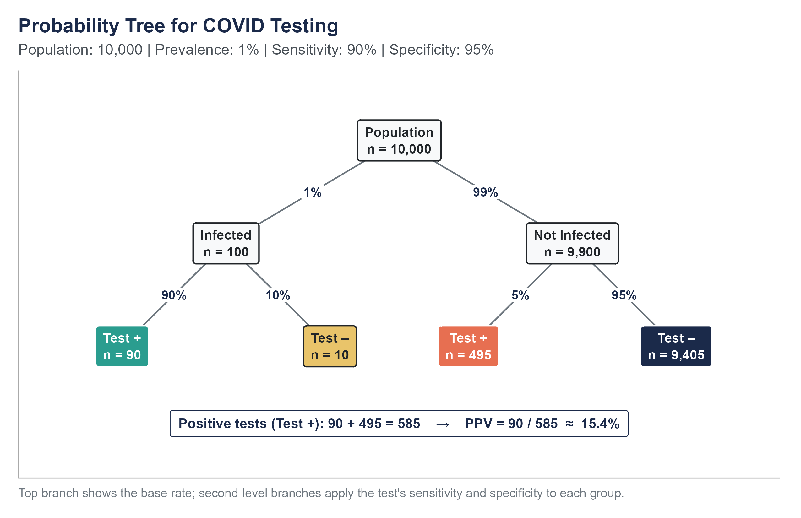
To find \(P(\text{infected} \mid \text{positive})\), look at all the “Test +” leaves. There are \(90 + 495 = 585\) positive tests. Of those, 90 come from the “Infected” branch.
\[P(\text{infected} \mid \text{positive}) = \frac{90}{90 + 495} = \frac{90}{585} \approx 0.154\]
The tree makes the structure visible. You can see that the false positive branch (495) dwarfs the true positive branch (90) because the “Not Infected” group is so much larger to begin with.
5.5.4 What Happens When the Base Rate Changes
The base rate is the engine that drives the result. Watch what happens when the prevalence changes but the test stays the same.
Scenario 1. Prevalence = 1% (our original scenario).
\(P(\text{infected} \mid \text{positive}) = 90 / 585 \approx 15.4\%\)
Scenario 2. Prevalence = 10%. Now 1,000 are infected and 9,000 are not.
True positives: \(1,000 \times 0.90 = 900\). False positives: \(9,000 \times 0.05 = 450\). Total positives: 1,350.
\(P(\text{infected} \mid \text{positive}) = 900 / 1,350 \approx 66.7\%\)
Scenario 3. Prevalence = 50%. Now 5,000 are infected and 5,000 are not.
True positives: \(5,000 \times 0.90 = 4,500\). False positives: \(5,000 \times 0.05 = 250\). Total positives: 4,750.
\(P(\text{infected} \mid \text{positive}) = 4,500 / 4,750 \approx 94.7\%\)
The same test. The same sensitivity. The same specificity. But the meaning of a positive result changes substantially depending on how common the disease is in the population being tested. This is why mass screening programs for rare diseases must be designed with extreme care, and why public health officials recommended against certain widespread testing strategies during COVID-19 when community prevalence was very low.
There is a practical lesson here for how testing was deployed during the pandemic. If you were a healthcare worker in a COVID ward, your exposure risk was high, the effective “base rate” for you was much higher than 1%. A positive test in that context was much more likely to be correct. If you were working from home in a rural area with very few cases, the same positive test was much more likely to be a false alarm. The test itself did not change. Your situation did. Probability is always conditional on context.
This is also why confirmatory testing is standard practice in medicine. A positive result on a screening test is usually followed up with a second, often more specific, test. The logic is Bayesian. Once someone tests positive on the first test, their updated probability of having the disease (the posterior probability) becomes the new base rate for interpreting the second test. If the first test raised the probability from 1% to 15%, and the second test is also positive, the probability climbs much higher. Two independent tests agreeing is far more informative than either test alone.
Return to the Base Rate Lab with everything you now know about Bayes’ theorem. Three tabs reinforce what you just read.
- Three Views puts the classical outcome-counting, frequentist long-run simulation, and Bayesian prior-to-posterior pictures side by side for the same problem. All three give the same PPV; they just get there by different mental routes.
- Scenarios lets you cycle through preset real-world tests (COVID rapid, screening mammography, HIV ELISA, workplace drug testing, airport behavioral screening, home pregnancy). Guess the PPV before you look, then compare. Low base rates are where intuition breaks most dramatically.
- Sequential Testing implements exactly the confirmatory-testing logic above: the posterior after test 1 becomes the prior for test 2. Watch how two independent positives can push the COVID probability from 1% to 15% and then to 77%.
Every diagnostic test has two types of errors. A false positive tells a healthy person they are sick. A false negative tells a sick person they are healthy. No test eliminates both.
Here is the ethical tension. Different stakeholders experience these errors differently.
For the individual tested during COVID-19, a false positive might have meant a two-week quarantine away from family, lost wages, missed school, and considerable anxiety, all for a disease they did not have. For someone who relied on hourly wages and had no paid sick leave, the cost was beyond psychological; it was financial.
For the community, a false negative was arguably worse. A person told they were not infected might have continued going to work, visiting elderly relatives, and spreading a virus they did not know they carried. One false negative could seed an outbreak.
For the employer, the calculus depended on the industry. A hospital administrator might have preferred more false positives (better to over-quarantine staff than risk an outbreak on the ward). A warehouse manager facing a labor shortage might have felt differently.
These tradeoffs are more than technical. They are moral. When public health agencies set the threshold for what counts as a “positive” result, they are implicitly making a value judgment about which type of error is more acceptable. Making that judgment transparent, rather than hiding it behind technical language, is an ethical obligation. Probability gives us the tools to quantify the tradeoffs. It does not tell us which tradeoff to choose. That is a human decision, and it should be made openly.
Large language models and AI systems can be very good at many tasks, but they sometimes stumble on exactly the kind of probabilistic reasoning we have been discussing.
When researchers have posed classic Bayesian reasoning problems to large language models, the results have been sobering. Binz and Schulz (2023), in a study published in the Proceedings of the National Academy of Sciences, ran a battery of cognitive psychology tasks against GPT-3 and found the same base-rate neglect that has been documented in humans for half a century. Macmillan-Scott and Musolesi (2024) extended this to seven different LLMs, including GPT-4 and Claude, and reported that none of them reasoned consistently well on standard probability tasks; their failures were not even consistent in the same direction across runs. A typical failure mode looks like this. When asked, “A disease affects 1 in 1,000 people. A test has a 5% false positive rate and a 99% true positive rate. If someone tests positive, what is the probability they have the disease?”, some models confidently answered “99%” or “95%”, committing the same confusion of the inverse that trips up humans. The correct answer, by Bayes’ theorem, is closer to 2%.
The issue is subtle. These models have seen Bayes’ theorem in their training data. They can recite the formula. They can sometimes solve textbook problems that are formatted in familiar ways. But when the problem is rephrased, or when the base rate is not highlighted, or when the question is embedded in a realistic scenario, they can fall back on the same heuristic that humans use. They match the answer to whichever number “feels” like it should be the answer, usually the sensitivity or the specificity.
This matters because AI tools are increasingly used in medical, legal, and financial contexts where base rates carry real weight. If you ask an AI assistant, “My patient tested positive on a screening test with 95% sensitivity and 90% specificity. The disease prevalence is 2%. Should I be concerned?”, you need the system to walk through the Bayesian calculation, not just report the sensitivity. As of this writing, some systems do this well and some do not, and the user has no easy way to tell the difference without understanding the math themselves.
The lesson is not “do not use AI for probability.” The lesson is that your understanding of base rates and conditional probability is your defense against both your own intuitive errors and the errors of any tool you rely on.
5.6 Random Variables and Expected Value
5.6.1 Random Variables
We have been talking about events, things like “rolling a 6” or “testing positive.” A random variable takes this a step further by assigning a numerical value to each outcome of a random process.
A random variable is typically denoted by a capital letter like \(X\). The specific values it can take are denoted by lowercase letters.
Example. Let \(X\) be the number of heads in three coin flips. The possible values of \(X\) are 0, 1, 2, and 3.
Example. Let \(Y\) be the number of points scored by a basketball team in a game. \(Y\) could be any non-negative integer, though in practice it falls within a certain range.
Example. Let \(Z\) be the time (in minutes) a customer waits on hold before reaching a service representative. \(Z\) can take any positive real value.
A discrete random variable takes on a countable number of values (like the number of heads, or the number of defective items in a batch). A continuous random variable can take any value within an interval (like waiting time, or temperature). This chapter focuses on discrete random variables. We will tackle continuous ones in the next chapter.
Why bother with the concept of a random variable when we were doing fine with events? Because random variables let us bring the tools of algebra and calculus to bear on probability. Once we assign numbers to outcomes, we can compute averages, measure spread, plot distributions, and build mathematical models. The language of random variables is the bridge between the probability rules we have learned and the statistical methods we will develop in the coming chapters.
5.6.2 Probability Distributions
A probability distribution for a discrete random variable specifies the probability of each possible value. It must satisfy two conditions: every probability is between 0 and 1, and all probabilities sum to 1.
For \(X\) = number of heads in three flips of a fair coin, the distribution is
| \(x\) | 0 | 1 | 2 | 3 |
|---|---|---|---|---|
| \(P(X = x)\) | \(1/8\) | \(3/8\) | \(3/8\) | \(1/8\) |
Where do these come from? With three flips, there are \(2^3 = 8\) equally likely outcomes (HHH, HHT, HTH, THH, HTT, THT, TTH, TTT). One outcome has 0 heads, three have exactly 1 head, three have exactly 2 heads, and one has 3 heads.
5.6.3 Expected Value
The expected value (or mean) of a discrete random variable \(X\) is the weighted average of its possible values, with the probabilities serving as weights.
\[E(X) = \sum_{i} x_i \cdot P(X = x_i)\]
For our coin-flip example,
\[E(X) = 0 \times \frac{1}{8} + 1 \times \frac{3}{8} + 2 \times \frac{3}{8} + 3 \times \frac{1}{8} = 0 + \frac{3}{8} + \frac{6}{8} + \frac{3}{8} = \frac{12}{8} = 1.5\]
You cannot flip 1.5 heads, of course. The expected value is not a prediction of any single outcome. It is the long-run average. If you repeated the three-flip experiment thousands of times and recorded the number of heads each time, the average of all those numbers would approach 1.5.
Example. A small insurance company offers a one-year policy that pays \(\$50{,}000\) if the policyholder is hospitalized during the year. Based on actuarial data, the probability of hospitalization is 0.02. The company charges \(\$1{,}200\) per policy. What is the expected profit per policy?
Let \(X\) be the company’s profit on a single policy.
- If no hospitalization (probability 0.98), the company collects \(\$1{,}200\) and pays nothing. Profit = \(\$1{,}200\).
- If hospitalization (probability 0.02), the company collects \(\$1{,}200\) and pays \(\$50{,}000\). Profit = \(\$1{,}200 - \$50{,}000 = -\$48{,}800\).
\[E(X) = 1{,}200 \times 0.98 + (-48{,}800) \times 0.02 = 1{,}176 - 976 = \$200\]
On average, the company expects to make \(\$200\) per policy. This does not mean every policy is profitable. Some will result in large payouts. But across a large number of policies, the average profit per policy should be near \(\$200\).
5.6.4 Variance and Standard Deviation of a Random Variable
The expected value tells us the center of a distribution, but not how spread out the values are. The variance of a random variable measures that spread.
\[\text{Var}(X) = E\left[(X - \mu)^2\right] = \sum_i (x_i - \mu)^2 \cdot P(X = x_i)\]
where \(\mu = E(X)\).
The standard deviation is the square root of the variance, \(\text{SD}(X) = \sqrt{\text{Var}(X)}\), and it has the same units as the original variable.
For the insurance example with \(E(X) = 200\),
\[\text{Var}(X) = (1{,}200 - 200)^2 \times 0.98 + (-48{,}800 - 200)^2 \times 0.02\] \[= (1{,}000)^2 \times 0.98 + (-49{,}000)^2 \times 0.02\] \[= 1{,}000{,}000 \times 0.98 + 2{,}401{,}000{,}000 \times 0.02\] \[= 980{,}000 + 48{,}020{,}000 = 49{,}000{,}000\]
\[\text{SD}(X) = \sqrt{49{,}000{,}000} = \$7{,}000\]
The expected profit is \(\$200\), but the standard deviation is \(\$7{,}000\). This tells us that the outcome on any individual policy is highly variable, even though the long-run average is positive. This is exactly why insurance companies need a large pool of policyholders. The individual outcomes are volatile, but the average across many policies stabilizes around the expected value, a phenomenon we will formalize later as the law of large numbers.
5.7 The Binomial Distribution
5.7.1 When Binomial Applies
Many real-world situations share a common structure. You repeat the same basic trial multiple times, each trial has only two possible outcomes (success or failure), the probability of success stays the same from trial to trial, and the trials are independent of each other.
Some examples that fit this structure (at least approximately):
- A free-throw shooter attempts 20 shots during a game. Each shot either goes in (success) or does not (failure).
- A quality inspector examines 50 items from a production line. Each item is either defective (success, if you are counting defects) or acceptable.
- A pollster contacts 500 registered voters. Each voter either supports a particular candidate (success) or does not.
- A pharmaceutical company enrolls 200 patients in a trial. Each patient either experiences a side effect or does not.
When these four conditions are met (fixed number of trials, two outcomes per trial, constant probability of success, independence), the number of successes follows a binomial distribution.
A brief note on the word “success.” In the context of the binomial distribution, “success” does not mean something good happened. It simply means the outcome you are counting occurred. If you are counting defective items, a defective item is a “success.” If you are counting patients who experience an adverse reaction, an adverse reaction is a “success.” The terminology is unfortunate, but it is standard, and you will encounter it everywhere.
5.7.2 The Binomial Formula
If \(X\) is the number of successes in \(n\) independent trials, each with probability of success \(p\), then
\[P(X = k) = \binom{n}{k} p^k (1-p)^{n-k}\]
for \(k = 0, 1, 2, \ldots, n\).
Let’s unpack each piece.
\(\binom{n}{k}\) is the binomial coefficient, read “n choose k.” It counts the number of ways to choose which \(k\) of the \(n\) trials will be the successes. The formula is
\[\binom{n}{k} = \frac{n!}{k!(n-k)!}\]
where \(n! = n \times (n-1) \times (n-2) \times \cdots \times 2 \times 1\) is the factorial of \(n\), with \(0! = 1\) by convention.
\(p^k\) is the probability of getting success on each of the \(k\) successful trials.
\((1-p)^{n-k}\) is the probability of getting failure on each of the remaining \(n-k\) trials.
The logic here is straightforward once you see it. Any particular sequence of \(k\) successes and \(n-k\) failures has probability \(p^k(1-p)^{n-k}\), because the trials are independent and you multiply probabilities. But there are \(\binom{n}{k}\) different orderings that produce exactly \(k\) successes. Since these orderings are mutually exclusive (only one can happen), we add them up, which is the same as multiplying \(\binom{n}{k}\) by the probability of any single arrangement.
5.7.3 A Worked Example
Suppose a basketball player has a 75% free-throw percentage, and they attempt 8 free throws in a game. What is the probability they make exactly 6?
Here \(n = 8\), \(k = 6\), \(p = 0.75\).
\[\binom{8}{6} = \frac{8!}{6! \cdot 2!} = \frac{8 \times 7}{2 \times 1} = 28\]
\[P(X = 6) = 28 \times (0.75)^6 \times (0.25)^2\]
\[= 28 \times 0.17798 \times 0.0625\]
\[= 28 \times 0.01112\]
\[\approx 0.3115\]
There is about a 31% chance they make exactly 6 of 8 free throws.
What about the probability they make 6 or more? That means \(P(X \geq 6) = P(X = 6) + P(X = 7) + P(X = 8)\).
\(P(X = 7) = \binom{8}{7}(0.75)^7(0.25)^1 = 8 \times 0.13348 \times 0.25 \approx 0.2670\)
\(P(X = 8) = \binom{8}{8}(0.75)^8(0.25)^0 = 1 \times 0.10011 \times 1 \approx 0.1001\)
\(P(X \geq 6) \approx 0.3115 + 0.2670 + 0.1001 = 0.6786\)
There is about a 68% chance they make 6 or more of their 8 free throws.
5.7.4 Mean and Standard Deviation of the Binomial
The expected value and standard deviation of a binomial random variable have particularly simple formulas.
\[E(X) = np\]
\[\text{SD}(X) = \sqrt{np(1-p)}\]
For our free-throw shooter, \(E(X) = 8 \times 0.75 = 6\) and \(\text{SD}(X) = \sqrt{8 \times 0.75 \times 0.25} = \sqrt{1.5} \approx 1.22\).
On average, they would make 6 out of 8, with a standard deviation of about 1.22. So making 5 or 7 (within about one standard deviation of the mean) would be completely unsurprising, while making 2 (more than three standard deviations below the mean) would be very unusual.
5.7.5 Building Intuition
Let’s use the binomial distribution to think about something more consequential. Suppose a new drug has a 40% response rate. A doctor prescribes it to 10 patients. What is the probability that none of them respond?
\[P(X = 0) = \binom{10}{0}(0.40)^0(0.60)^{10} = 1 \times 1 \times 0.006047 \approx 0.006\]
About 0.6%. Very unlikely, which is reassuring if you are the drug manufacturer. But let’s turn this around. What is the probability that fewer than 3 patients respond?
\[P(X < 3) = P(X = 0) + P(X = 1) + P(X = 2)\]
\(P(X = 0) \approx 0.006\)
\(P(X = 1) = \binom{10}{1}(0.40)^1(0.60)^9 = 10 \times 0.40 \times 0.01008 \approx 0.040\)
\(P(X = 2) = \binom{10}{2}(0.40)^2(0.60)^8 = 45 \times 0.16 \times 0.01680 \approx 0.121\)
\(P(X < 3) \approx 0.006 + 0.040 + 0.121 = 0.167\)
About a 17% chance. So even with a drug that works 40% of the time, a doctor treating 10 patients has a non-trivial chance of seeing fewer than 3 responses. This is important context for clinical decision-making. A doctor who sees only 2 of 10 patients respond might lose confidence in the drug, but the binomial distribution tells us this outcome is not that unusual. Small samples produce noisy results.
This connects to one of the deepest themes in statistics. Variability in small samples does not mean something is broken. It means you need more data before drawing conclusions.
Open the Binomial Explorer on the companion website. Set \(n\) and \(p\) with the sliders and watch the PMF update live. Three things to do before you move on.
- Distribution tab. Reproduce the free-throw example: set \(n = 8\), \(p = 0.75\), and choose the highlight \(P(X = k)\) with \(k = 6\). The bar chart should show the same 0.3115 we computed by hand. Then switch the highlight to \(P(X \geq k)\) to see the 0.6786 from the next paragraph.
- Shape Lab tab. Hold \(p\) fixed at 0.30 and step \(n\) through 10, 30, and 100. Watch the bars become smoother and more symmetric: a preview of the Central Limit Theorem in Chapter 6.
- Calculator tab. Pick any \((n, p)\) and find the smallest \(k\) with \(P(X \leq k) \geq 0.95\). That’s the 95th percentile of the distribution, the same idea that will show up in confidence intervals in Chapter 7.
5.7.6 When the Binomial Does Not Apply
It is worth being clear about when the binomial model breaks down, because forcing data into the wrong model produces misleading results.
Trials are not independent. If you are drawing cards from a deck without replacement, each draw changes the composition of the remaining deck. The probability of drawing a heart on the second card depends on what happened on the first draw. For small samples from large populations, the dependence is negligible and the binomial is a reasonable approximation. But for larger samples, or for populations that are not much larger than the sample, you need a different distribution (the hypergeometric, which we will not cover in this book but which you may encounter in more advanced work).
The probability of success changes. If a salesperson’s probability of closing a deal improves as they gain experience throughout the day, the constant-probability assumption is violated. If the probability of a manufacturing defect increases as a machine wears out over a shift, same problem.
More than two outcomes. If each trial can result in three or more categories (a customer chooses brand A, brand B, or brand C), the binomial does not apply directly. You would need its generalization, the multinomial distribution.
Recognizing when a model fits and when it does not is just as important as knowing how to use the model when it does fit.
5.8 Tying It Together
Let’s return once more to where we started. The COVID testing scenario is ultimately a story about conditional probability, Bayes’ theorem, and the power of base rates. But it also involves every concept in this chapter.
The test result is a random variable (positive or negative). The probability rules let us combine the base rate with the test characteristics. The complement rule reminds us that \(P(\text{not infected}) = 1 - P(\text{infected})\). The multiplication rule connects the joint probability of being infected and testing positive to the conditional probability of testing positive given infection. And Bayes’ theorem ties the whole calculation together, allowing us to flip the conditional probability from what the test tells us to what we actually want to know.
If you take away one idea from this chapter, let it be this. Probabilities are not isolated numbers. They exist in context. A 90% accuracy rate means different things depending on what you are testing for, who you are testing, and how common the condition is. Understanding probability is not about memorizing formulas, though the formulas are useful. It is about developing the habit of asking, “What is the full picture? What other information do I need before I can interpret this number?”
That habit of mind, thinking carefully about context and conditions, is the foundation of every statistical method we will build in the rest of this book.
And it is a habit that transfers far beyond statistics. In business, in medicine, in policy, in your personal decisions, the question “what is the base rate?” is almost always the right starting point. Before you get excited about a positive result, ask how common the thing you are looking for is in the first place. Before you panic about a risk, ask how frequently that risk materializes in the relevant population. Before you trust a prediction, ask what the prior probability was before the evidence arrived.
Probability is more than a mathematical tool. It is a way of thinking carefully about uncertainty. And in a world full of uncertainty, thinking carefully is never wasted effort.
5.9 Looking Ahead
Everything in this chapter has dealt with discrete outcomes: events you can list and count, like coin flips, test results, or the number of defective items in a batch. But many real-world quantities, such as height, weight, income, or time, are continuous. For a continuous random variable, the probability of observing any single exact value is zero; instead, we calculate probabilities over ranges. That shift from counting outcomes to measuring areas under a curve is the subject of the next chapter, where we meet the most important continuous distribution in statistics: the normal distribution. Along the way, we will encounter the Empirical Rule, z-scores, and ultimately the Central Limit Theorem, the result that makes nearly all of statistical inference possible.
5.10 Further Reading and References
The following works are cited in this chapter or provide valuable additional context for the ideas covered here.
On Bayes’ theorem and natural frequencies: Gigerenzer, G. (2002). Calculated risks: How to know when numbers deceive you. Simon & Schuster. (An accessible treatment of how natural frequency representations, like the 10,000-person table used in this chapter, help people reason about conditional probability far more accurately than traditional probability notation.)
Gigerenzer, G., & Hoffrage, U. (1995). How to improve Bayesian reasoning without instruction: Frequency formats. Psychological Review, 102(4), 684–704. (The research paper demonstrating that physicians and laypeople alike perform dramatically better on Bayesian reasoning tasks when information is presented as natural frequencies rather than conditional probabilities.)
On the base rate fallacy: Kahneman, D., & Tversky, A. (1973). On the psychology of prediction. Psychological Review, 80(4), 237–251. (The foundational paper documenting how people systematically ignore base rates when making probabilistic judgments.)
On COVID-19 testing and probabilistic reasoning: Watson, J., Whiting, P. F., & Brush, J. E. (2020). Interpreting a COVID-19 test result. BMJ, 369, m1808. (A clear explanation of positive predictive value, sensitivity, specificity, and prevalence applied to COVID-19 testing, closely paralleling the scenario that opens this chapter.)
For further reading on probability: Blitzstein, J. K., & Hwang, J. (2019). Introduction to probability (2nd ed.). CRC Press. (A thorough, example-driven probability textbook that develops the concepts introduced in this chapter at much greater depth, with applications across disciplines.)
Gigerenzer, G., Gaissmaier, W., Kurz-Milcke, E., Schwartz, L. M., & Woloshin, S. (2007). Helping doctors and patients make sense of health statistics. Psychological Science in the Public Interest, 8(2), 53–96. (A comprehensive review of how statistical illiteracy among both physicians and patients leads to poor health decisions, extending the natural-frequencies approach introduced in this chapter.)
On large language models and probabilistic reasoning: Binz, M., & Schulz, E. (2023). Using cognitive psychology to understand GPT-3. Proceedings of the National Academy of Sciences, 120(6), e2218523120. (Documents that GPT-3 reproduces several classic human reasoning biases, including base-rate neglect, on standard cognitive psychology tasks.)
Macmillan-Scott, O., & Musolesi, M. (2024). (Ir)rationality and cognitive biases in large language models. Royal Society Open Science, 11(6), 240255. (Tests seven large language models on classic probability and reasoning problems and finds that none reason consistently well, with failures that vary even across repeated runs of the same prompt.)
5.11 Key Terms
- Sample space (\(S\)): The set of all possible outcomes of a random process.
- Event: A subset of the sample space, representing one or more outcomes of interest.
- Probability: A number between 0 and 1 that measures how likely an event is to occur.
- Complement: The complement of event \(A\), written \(A^c\), is the event that \(A\) does not occur. \(P(A^c) = 1 - P(A)\).
- Mutually exclusive events: Events that cannot occur at the same time. \(P(A \text{ and } B) = 0\).
- Addition rule: \(P(A \text{ or } B) = P(A) + P(B) - P(A \text{ and } B)\).
- Independent events: Events where the occurrence of one does not affect the probability of the other. \(P(A \text{ and } B) = P(A) \times P(B)\).
- Conditional probability: The probability of \(A\) given that \(B\) has occurred, \(P(A \mid B) = P(A \text{ and } B) / P(B)\).
- Bayes’ theorem: \(P(A \mid B) = P(B \mid A) \times P(A) / P(B)\). Allows us to update probabilities in light of new evidence.
- Base rate: The overall probability of a condition in the population, before any test or evidence is considered.
- Sensitivity: \(P(\text{positive test} \mid \text{disease present})\). The probability that a test correctly identifies someone who has the condition.
- Specificity: \(P(\text{negative test} \mid \text{disease absent})\). The probability that a test correctly identifies someone who does not have the condition.
- Positive predictive value: \(P(\text{disease present} \mid \text{positive test})\). The probability that someone with a positive test actually has the condition.
- False positive: A test result that says the condition is present when it is not.
- False negative: A test result that says the condition is absent when it is present.
- Natural frequencies: Presenting probability information as counts in a hypothetical population (e.g., “out of 10,000 people”) rather than as percentages. Tends to improve human reasoning.
- Random variable: A numerical quantity whose value is determined by a random process.
- Probability distribution: A specification of all possible values of a random variable and their associated probabilities.
- Expected value: The long-run average of a random variable, calculated as \(E(X) = \sum x_i \cdot P(X = x_i)\).
- Variance: A measure of how spread out the values of a random variable are around the expected value.
- Binomial distribution: The distribution of the number of successes in \(n\) independent trials, each with success probability \(p\). \(P(X = k) = \binom{n}{k} p^k (1-p)^{n-k}\).
- Binomial coefficient: \(\binom{n}{k} = n! / [k!(n-k)!]\). The number of ways to choose \(k\) items from \(n\).
- Law of total probability: \(P(B) = P(B \mid A) \times P(A) + P(B \mid A^c) \times P(A^c)\). Allows us to compute the overall probability of \(B\) by considering all the ways \(B\) can occur.
- Confusion of the inverse: The error of treating \(P(A \mid B)\) as if it were \(P(B \mid A)\).
- Continuous random variable: A random variable that can take any value within an interval, such as height or temperature. Covered in detail in Chapter 6.
- Discrete random variable: A random variable that takes on a countable number of values, such as the number of heads in ten coin flips.
- Prosecutor’s fallacy: The error of treating \(P(A \mid B)\) as if it were \(P(B \mid A)\), particularly dangerous in legal and medical contexts.
A full R walkthrough of this chapter is online at stats.marginoferrormedia.com/walkthroughs/r-ch05.html. It computes sensitivity, specificity, PPV, and Bayes’ theorem on the COVID test data, plus the binomial PMF and a PPV-vs-prevalence curve.
5.12 Exercises
5.12.1 Check Your Understanding
These questions test whether you have grasped the core concepts. You should be able to answer them without extensive calculation.
1. A weather app says there is a 30% chance of rain tomorrow. What is the probability it does not rain?
2. Are the events “a student is left-handed” and “a student is right-handed” mutually exclusive? Are they exhaustive (do they cover all possibilities)? Explain.
3. A bag contains 5 red marbles and 3 blue marbles. You draw one marble. Are the events “draw a red marble” and “draw a blue marble” independent? Are they mutually exclusive? Explain the difference between these two concepts.
4. In your own words, explain why \(P(\text{disease} \mid \text{positive test})\) is not the same as \(P(\text{positive test} \mid \text{disease})\). Give a non-medical example that illustrates the same idea.
5. A test has 99% sensitivity and 95% specificity. The disease prevalence is 0.1%. Without doing a formal calculation, explain whether you would expect the positive predictive value to be high or low, and why.
6. Suppose \(P(A) = 0.4\), \(P(B) = 0.5\), and \(P(A \text{ and } B) = 0.2\). Are \(A\) and \(B\) independent? How do you know?
7. What does it mean to say that two events are independent? Give an example of two events that are independent and two events that are not.
8. Why does the expected value of a random variable not have to be a value the variable can actually take? Illustrate with an example.
9. List the four conditions that must be satisfied for a situation to follow a binomial distribution. For each condition, give an example of a situation where that particular condition would be violated.
10. A friend says, “My coin came up heads five times in a row, so it is due for tails.” What concept from this chapter does your friend misunderstand? Explain.
5.12.2 Apply It
These problems require calculations. Show your work and interpret your results in context.
1. A company’s records show that 60% of its employees have a college degree, 45% have more than five years of experience, and 30% have both. What is the probability that a randomly selected employee has a college degree or more than five years of experience (or both)?
2. At a large hospital, 8% of patients are admitted to the ICU. Among ICU patients, 20% require mechanical ventilation. Among non-ICU patients, 1% require mechanical ventilation. What is the probability that a randomly selected patient requires mechanical ventilation?
3. Using the hospital data from problem 2, if a patient is on mechanical ventilation, what is the probability they are in the ICU? Use Bayes’ theorem or a frequency table approach.
4. A rapid strep test has a sensitivity of 86% and a specificity of 95%. In a pediatric clinic during winter, the prevalence of strep throat among children presenting with sore throat is about 30%. A child tests positive. What is the probability they actually have strep throat? Construct a frequency table using a hypothetical population of 1,000 children to find your answer.
5. A quality control process involves inspecting 15 items from each production batch. Historical data shows a 3% defect rate. Let \(X\) be the number of defective items in a sample of 15.
What is the probability that the sample contains no defective items?
What is the probability that the sample contains exactly one defective item?
What is the probability that the sample contains two or more defective items?
What are the expected value and standard deviation of \(X\)?
6. Two independent fire alarms are installed in a building. During a fire, alarm A activates with probability 0.95 and alarm B activates with probability 0.90.
What is the probability both alarms activate during a fire?
What is the probability neither alarm activates? (This is the scenario the building manager worries about most.)
What is the probability at least one alarm activates?
7. A genetic screening test for a rare condition has the following characteristics. Sensitivity is 99.5% and specificity is 99%. The condition affects 1 in 5,000 newborns. In a city with 20,000 births per year, how many positive test results would you expect? How many of those would be true positives? Calculate the positive predictive value.
8. A small business owner sells handmade candles at a farmer’s market. On any given Saturday, the probability of selling 0 candles is 0.05, selling 1-5 candles is 0.20, selling 6-10 candles is 0.40, selling 11-15 candles is 0.25, and selling more than 15 candles is 0.10. The owner makes a profit of \(\$5\) per candle but pays \(\$30\) to rent the booth. Using the midpoints of each range (0, 3, 8, 13, 18), find the expected number of candles sold and the expected profit.
9. A recent survey found that 72% of adults in a city support expanding public transit. You randomly sample 12 adults from this city.
What is the probability that exactly 9 support the expansion?
What is the probability that 10 or more support the expansion?
What is the expected number of supporters in your sample?
Would it be unusual to find that only 5 of the 12 support the expansion? Justify your answer using the mean and standard deviation.
10. Two events \(A\) and \(B\) satisfy \(P(A) = 0.3\), \(P(B \mid A) = 0.6\), and \(P(B \mid A^c) = 0.2\).
Find \(P(A \text{ and } B)\).
Find \(P(B)\) using the law of total probability.
Find \(P(A \mid B)\) using Bayes’ theorem.
Are \(A\) and \(B\) independent? Explain.
The following three exercises use the covid-testing.csv dataset available on the companion website. This is a simulated dataset mathematically modeled to reflect real-world patterns from published sensitivity and specificity estimates for diagnostic tests during the COVID-19 pandemic. No real patients are represented. The dataset contains 2,000 observations with variables including patient_id, truly_infected (Yes/No), test_result (Positive/Negative), age_group (18–29, 30–44, 45–59, 60–74, 75+), and risk_category (Low/Medium/High).
11. Using the covid-testing.csv dataset, construct a \(2 \times 2\) frequency table of truly_infected (rows) versus test_result (columns). From this table, calculate the sensitivity (true positive rate) and specificity (true negative rate) of the test. Then calculate the positive predictive value: among all patients who tested positive, what proportion were truly infected? Compare this value to the sensitivity and explain why they differ.
12. Compute the prevalence of infection (proportion with truly_infected = Yes) separately for each age_group. Display these five proportions in a table. Which age group has the highest prevalence? Now compute the positive predictive value for each age group separately (among those who tested positive within each age group, what fraction were truly infected?). How does PPV change across age groups, and why? Connect your answer to Bayes’ theorem.
13. Restrict your analysis to the High risk category only. Within this subgroup, construct a new \(2 \times 2\) frequency table of infection status versus test result. Calculate the prevalence, sensitivity, specificity, and positive predictive value for this subgroup. Compare these values to the overall values you computed in Problem 11. Does the test perform differently in a high-risk population? Explain why or why not, using the concepts of base rate and Bayes’ theorem.
5.12.3 Think Deeper
These questions ask you to reflect on the concepts in broader context. There is not always a single correct answer.
1. During the early months of COVID-19, many workplaces required employees to test negative before returning to work. Using what you have learned about base rates and predictive values, discuss the strengths and limitations of this policy. Under what conditions (in terms of prevalence, test sensitivity, and specificity) would such a policy be most effective? Under what conditions might it cause more harm than good?
2. In criminal trials, forensic evidence is sometimes presented with statements like “the probability of finding this DNA match if the defendant were innocent is 1 in 10 million.” Explain why this statement does not mean “the probability that the defendant is innocent is 1 in 10 million.” What additional information would a juror need to properly evaluate this evidence? How does this connect to Bayes’ theorem?
3. Insurance companies use probability calculations to set premiums, as illustrated in the expected value example in this chapter. Some critics argue that using demographic data (such as age, gender, or zip code) to set different premiums for different groups amounts to discrimination, even if the probabilities are accurate. Others argue that charging everyone the same rate unfairly forces low-risk groups to subsidize high-risk groups. Where do you stand on this issue? What role should probability and statistical risk assessment play in decisions that affect individuals? Are there cases where actuarially accurate pricing should be overridden by other considerations?
4. Consider two screening tests for the same disease. Test A has 99% sensitivity and 90% specificity. Test B has 90% sensitivity and 99% specificity. The disease prevalence is 2%.
Calculate the positive predictive value and negative predictive value for each test.
If this disease is fatal when undetected, which test would you prefer for screening? Why?
If the treatment for this disease has severe side effects, which test would you prefer? Why?
What does this exercise reveal about the claim that one test is “better” than another?
5. Gigerenzer and colleagues have shown that presenting probability information as natural frequencies substantially improves people’s ability to reason about Bayesian problems. Yet most medical test results are still communicated to patients as percentages (“this test has a 95% accuracy rate”). Why do you think the medical establishment has been slow to adopt frequency-based communication? What are the potential consequences of this communication gap? If you were designing a patient-facing health app that reported test results, how would you present the information?