11 Multiple Regression

11.1 The Question That Launched a Thousand Arguments

In the 1985 Current Population Survey data used throughout this chapter, the average hourly wage for women working full-time was about 78.8% of men’s wages. This means that for every dollar earned by the average man, the average woman earned about 79 cents.

That number, the raw gender wage gap, is among the most-argued statistics in American public life. The arguments almost always take the same form.

One side says the gap is evidence of discrimination. The other side says that once you “control for” occupation, experience, hours worked, education, and industry, the gap shrinks to a few cents or disappears entirely. The first side counters that you cannot control for occupation and still call the analysis fair, because the very occupations women end up in are shaped by discrimination. The second side says you cannot attribute to discrimination what is explained by choices.

Around and around it goes. And what almost nobody in the argument stops to do is ask the question that actually matters, the question this chapter will teach you to answer. When someone says they are “controlling for” a variable, what, precisely, are they doing? What does the math look like? What assumptions is the analysis making? And when are those assumptions reasonable versus dangerously misleading?

The tool at the center of this debate is multiple regression. It is widely used across empirical social science, business analytics, public health research, and increasingly, everyday journalism. It lets you model the relationship between an outcome and several predictors simultaneously, which is what people mean when they say they are “controlling for” things. Understanding what it can and cannot do is a foundational form of statistical literacy.

Let us build that understanding from the ground up.

11.2 From One Predictor to Many

In Chapter 10, we explored simple linear regression. We modeled the relationship between a single predictor variable $X$ and an outcome variable $Y$ using the equation

\[Y = b_0 + b_1 X + e\]

where $b_0$ is the intercept, $b_1$ is the slope, and $e$ is the sample-level residual — the part of $Y$ that the fitted line does not explain. The corresponding population-level equation, introduced in the Signal, Noise, and the Population Model section of Chapter 10, replaces $b_0, b_1, e$ with $\beta_0, \beta_1, \varepsilon$, where $\varepsilon$ is the unobservable random error. The same convention carries through this chapter: Greek letters for unknown population parameters, Latin for the sample estimates we actually compute.

If $X$ is years of work experience and $Y$ is annual salary, then $b_1$ tells you how much salary tends to change for each additional year of experience. The slope $b_1$ has units: dollars per year of experience. This will matter shortly when we discuss what coefficients mean.

But salary is not determined by experience alone. Education matters. Occupation matters. Geographic location matters. Union membership and other factors matter. If you want to understand salary, a model with one predictor is going to miss a lot.

Multiple regression addresses this by allowing more than one predictor variable in the model. The general form is

\[Y = b_0 + b_1 X_1 + b_2 X_2 + b_3 X_3 + \cdots + b_k X_k + e\]

where $k$ is the number of predictors. Each $b_j$ is a regression coefficient that tells you the estimated relationship between predictor $X_j$ and the outcome $Y$, while accounting for all the other predictors in the model. Each coefficient carries units: $b_j$ is in units of $Y$ per unit of $X_j$. If $Y$ is annual salary in dollars and $X_j$ is years of experience, $b_j$ is in dollars per year. If $X_j$ is a dummy variable (which is unitless, just 0 or 1), then $b_j$ is in units of $Y$ — for example, dollars. The unitless quantity from Chapter 4, the correlation $r$, is a different beast; raw regression coefficients keep the units of the variables they relate.

Suppose you model salary as a function of experience, education (measured in years of schooling), and weekly hours worked.

\[\text{Salary} = b_0 + b_1(\text{Experience}) + b_2(\text{Education}) + b_3(\text{Hours}) + e\]

If you fit this model to data and find $b_1 = 1,\!850$, that means each additional year of experience is associated with an estimated $1,850 increase in salary, after accounting for differences in education and hours worked. This is the “holding all other variables constant” interpretation, and it is both the great power and the great peril of multiple regression. We will dig into what it means, and what it does not mean, shortly.

11.2.1 How the Coefficients Are Estimated

The estimation procedure for multiple regression follows the same logic as simple regression. We find the set of coefficients $b_0, b_1, \ldots, b_k$ that minimizes the sum of squared residuals

\[\sum_{i=1}^{n} e_i^2 = \sum_{i=1}^{n} (Y_i - \hat{Y}_i)^2\]

where $\hat{Y}_i = b_0 + b_1 X_{1i} + b_2 X_{2i} + \cdots + b_k X_{ki}$ is the predicted value for observation $i$. This is still ordinary least squares (OLS, introduced in Chapter 10), just extended to more dimensions. The mathematics involves matrix algebra rather than the simple formulas from Chapter 10, but the principle is identical. Find the line, or more accurately the hyperplane, that makes the predictions as close to the actual values as possible, on average.

In simple regression, you are fitting a line through a cloud of points in two-dimensional space. In multiple regression with two predictors, you are fitting a plane through a cloud in three-dimensional space. With more predictors, you are fitting a surface in higher-dimensional space that you cannot visualize but that the math handles without complaint.

11.3 “Holding All Other Variables Constant”

This phrase is the most important thing to understand about multiple regression, and it is also the thing most likely to be misunderstood.

When we say that the coefficient on experience is $1,850 “holding education and hours constant,” we mean something very specific. We are comparing people who have the same education level and the same weekly hours, and asking how salary differs between those who have, say, 10 years of experience versus 11 years. Among people with equal education and equal hours, each extra year of experience is associated with about $1,850 more in salary.

This is not the same as the simple relationship between experience and salary. In a simple regression of salary on experience alone, you might get a coefficient of $2,400. The reason it differs is that experience is correlated with other variables. People with more experience often have more education. People with more experience might work longer hours. The simple regression lumps all of these effects together. Multiple regression tries to separate them.

The word “tries” is doing heavy lifting in that sentence. Multiple regression separates the effects to the extent that the model’s assumptions are met and the right variables are included. It cannot separate what it cannot see. If there is an important variable that affects salary and is correlated with experience, but you left it out of the model, then the coefficient on experience will absorb some of that missing variable’s effect. This is called omitted variable bias, and we will come back to it later in this chapter because it is a foundational concept for thinking critically about regression results.

For now, keep this in mind. “Holding all other variables constant” means “holding all other included variables constant.” It says nothing about variables not in the model.

Note

The phrase “controlling for” has become so common in popular writing that people use it almost casually. “After controlling for income, there is no difference in health outcomes between the two groups.” Statements like this can be accurate, but they are only as good as the model that produced them. When you see “after controlling for” in a news article or a research summary, your first question should be, “What exactly was controlled for, and what was left out?” Your second question should be, “Are any of the control variables themselves affected by the thing we are studying?” We will explore this second question in the ethics section of this chapter.

11.4 Categorical Predictors and Dummy Variables

So far, we have talked about predictors that are numerical, like years of experience or hours worked. But many central predictors in social science and business are categorical. Gender. Race. Region of the country. Occupation. Job title. Department.

You cannot plug “female” into the equation $Y = b_0 + b_1 X_1$ as a number. So how do we include categorical variables in a regression model?

The answer is dummy variables, also called indicator variables. A dummy variable is a variable that takes the value 1 if a condition is true and 0 otherwise. To include gender (coded as male and female) in a regression model, you create a variable

\[\text{Female} = \begin{cases} 1 & \text{if the person is female} \\ 0 & \text{if the person is male} \end{cases}\]

A note on this coding before we go further. Treating gender as a binary variable here reflects how it was recorded in the 1985 Current Population Survey (and in most administrative data of that period), not a claim that gender is binary in fact. When working with a richer gender variable that includes nonbinary identities or self-described categories, you would create $k - 1$ dummy variables in the same way the next subsection describes for any categorical variable with $k$ levels. The mechanics of the regression do not change. Only the categories — and the care with which you describe them — do.

Then you include this variable in the model like any other predictor.

\[\text{Salary} = b_0 + b_1(\text{Experience}) + b_2(\text{Education}) + b_3(\text{Female}) + e\]

If $b_3 = -4,\!200$, that means women in this sample earn an estimated $4,200 less than men, after accounting for differences in experience and education. The group coded as 0, in this case men, is called the reference category. The coefficient on the dummy variable always represents the difference between the coded group and the reference group.

11.4.1 Categorical Variables with More Than Two Categories

What if you want to include a variable like occupation, with six categories: Manufacturing, Tech, Education, Healthcare, Finance, and Retail? You cannot represent this with a single variable coded 1 through 6, because that would imply that the occupations have a natural ordering and that the distance between Manufacturing and Tech is the same as between Tech and Education. That makes no sense.

Instead, you create $k - 1$ dummy variables, where $k$ is the number of categories. For six occupation categories, you create five dummies.

\[\text{Tech} = \begin{cases} 1 & \text{if Tech} \\ 0 & \text{otherwise} \end{cases} \quad \text{Education} = \begin{cases} 1 & \text{if Education} \\ 0 & \text{otherwise} \end{cases} \quad \text{Healthcare} = \begin{cases} 1 & \text{if Healthcare} \\ 0 & \text{otherwise} \end{cases}\]

\[\text{Finance} = \begin{cases} 1 & \text{if Finance} \\ 0 & \text{otherwise} \end{cases} \quad \text{Retail} = \begin{cases} 1 & \text{if Retail} \\ 0 & \text{otherwise} \end{cases}\]

Someone in Manufacturing would have all five dummies equal to 0. Manufacturing becomes the reference category. The coefficient on Tech tells you the average difference in the outcome between people in Tech and people in Manufacturing, holding everything else constant. The coefficient on Education tells you the Education-versus-Manufacturing difference. And so on.

Why $k - 1$ dummies instead of $k$? Because if you know that someone is not in Tech, not in Education, not in Healthcare, not in Finance, and not in Retail, you already know they are in Manufacturing. The sixth dummy is redundant, and including it would cause a mathematical problem called perfect multicollinearity (the columns of the design matrix would be linearly dependent, and the estimation procedure would break down). Most software handles this automatically, but it helps to understand why one category always goes missing from the output.

11.4.2 Choosing the Reference Category

The choice of reference category does not change the substance of the model. It only changes which comparisons show up directly in the coefficients. If you make Education the reference category instead of Manufacturing, the coefficients on the other occupation categories change, but the predicted values for every observation remain exactly the same.

That said, it is a good practice to choose a reference category that makes interpretation easy. Common choices include the most common group, the group that serves as a natural baseline, or the group that your audience is most likely to be comparing against.

11.5 Interaction Effects

So far, every model we have written assumes that the effect of each predictor is the same regardless of the values of the other predictors. Experience adds $1,850 to salary whether you are male or female, in Manufacturing or Finance, in Alabama or Alaska. That is a strong assumption, and it is often wrong.

An interaction effect occurs when the relationship between one predictor and the outcome depends on the value of another predictor. In the wage gap context, suppose the salary premium for each additional year of experience is larger for men than for women. That would mean gender and experience interact in their effect on salary.

To model this, you create an interaction term by multiplying the two predictors together and adding the product as a new variable.

\[\text{Salary} = b_0 + b_1(\text{Experience}) + b_2(\text{Female}) + b_3(\text{Experience} \times \text{Female}) + e\]

Now the effect of experience is not a single number. For men (Female = 0), each additional year of experience is associated with a $b_1$ increase in salary. For women (Female = 1), each additional year is associated with a $b_1 + b_3$ increase. The coefficient $b_3$ tells you how much the experience effect differs between men and women. If $b_3$ is negative, the returns to experience are smaller for women. If $b_3$ is positive, the returns are larger.

This matters for interpretation. A model without the interaction might show a $4,000 gender gap that looks constant across experience levels. A model with the interaction might reveal that the gap is small for recent graduates and grows with each year of experience, a very different story with very different policy implications.

A practical caution: interaction terms multiply the number of coefficients and can introduce multicollinearity (defined formally in the next major section), especially when the interacted variables are correlated. Include interactions when you have a substantive reason to believe the effect of one predictor depends on another. Do not include them routinely in every model.

11.6 R-Squared vs. Adjusted R-Squared

In Chapter 10, we introduced $R^2$ as a measure of how well the regression model fits the data. It tells you what proportion of the variance in the outcome is explained by the predictors. An $R^2$ of 0.45 means the model explains 45% of the variability in the outcome, with the remaining 55% unexplained.

Multiple regression introduces a subtlety. When you add a new predictor to a regression model, $R^2$ will go up, or at worst stay the same, even if the new predictor has no real relationship with the outcome. This is built into the algebra — every new predictor gives the model one more degree of freedom to chase the noise in the data, and $R^2$ rewards that chase. If you added random numbers as a predictor, $R^2$ would still go up (by a tiny amount).

This means $R^2$ is a poor guide for comparing models with different numbers of predictors. A model with 20 predictors will almost always have a higher $R^2$ than a model with 5 predictors, but that does not mean the 20-predictor model is better. Some of those 15 extra predictors might be adding noise, not signal.

Adjusted $R^2$ fixes this by penalizing the model for each additional predictor. The formula is

\[R^2_{adj} = 1 - \frac{(1 - R^2)(n - 1)}{n - k - 1}\]

where $n$ is the sample size and $k$ is the number of predictors. The penalty increases as you add predictors. If a new predictor does not improve the model enough to overcome the penalty, adjusted $R^2$ will actually go down. This makes adjusted $R^2$ a better tool for comparing models of different sizes.

A practical example. You model salary using experience alone and get $R^2 = 0.32$ and $R^2_{adj} = 0.319$. You add education and hours worked. Now $R^2 = 0.47$ and $R^2_{adj} = 0.465$. Both $R^2$ and adjusted $R^2$ went up, suggesting the additional predictors provide real improvement. You then add 15 more variables, including shoe size, number of vowels in the person’s last name, and birth month. Now $R^2 = 0.49$ but $R^2_{adj} = 0.441$. The adjusted $R^2$ went down, telling you that the additional variables are adding complexity without enough explanatory value to justify it.

Neither $R^2$ nor adjusted $R^2$ should be the sole criterion for model selection. They say nothing about whether the model’s assumptions are met, whether the coefficients are interpretable, or whether important variables were omitted. But adjusted $R^2$ is a useful early diagnostic for deciding whether a more complex model is pulling its weight.

11.7 Multicollinearity

Multiple regression works by separating the individual contributions of each predictor. But what happens when two or more predictors are highly correlated with each other? This situation is called multicollinearity, and it creates real problems for interpretation.

11.7.1 What It Is

Consider a model predicting salary from both “years of experience” and “age.” These two variables are highly correlated. Older people generally have more experience. When you put both in a regression, the model has a hard time telling which variable is driving the relationship with salary. Is salary going up because of experience, or because of age, or some mixture of both?

The math still works. The model will produce estimates. But the coefficients become unstable. Small changes in the data can cause large swings in the estimated coefficients. The standard errors of the coefficients become inflated, making it harder to detect statistically significant relationships. And the individual coefficients become difficult to interpret, because “holding age constant while increasing experience” is nearly impossible in reality, the two move together.

11.7.2 The Extreme Case

Perfect multicollinearity, where one predictor is an exact linear function of others, causes the estimation to fail entirely. The classic example is including dummy variables for all categories of a categorical variable (including the reference), which we discussed above. Another example would be including both “income in dollars” and “income in thousands of dollars” as separate predictors. Software will refuse to estimate the model or will drop one variable automatically.

11.7.3 Detecting Multicollinearity with VIF

The most common diagnostic for multicollinearity is the Variance Inflation Factor (VIF). The VIF for a predictor $X_j$ is calculated by regressing $X_j$ on all the other predictors and computing

\[\text{VIF}_j = \frac{1}{1 - R^2_j}\]

where $R^2_j$ is the R-squared from that auxiliary regression. A VIF of 1 means the predictor is not correlated with the others at all. A VIF of 5 means the variance of the coefficient is inflated by a factor of 5 due to correlation with other predictors. A VIF of 10 means tenfold inflation.

Common rules of thumb suggest concern when VIF exceeds 5, and serious concern when it exceeds 10. But these are guidelines, not laws. In some contexts, even a VIF of 3 can cause problems. In others, a VIF of 8 might be tolerable if you are not interested in interpreting the individual coefficient.

11.7.4 What To Do About It

If multicollinearity is a problem, your options include dropping one of the correlated predictors, combining correlated predictors into a single measure (for instance, creating an index), collecting more data (larger samples reduce the instability, though they do not eliminate it), or simply acknowledging that the individual coefficients for the correlated predictors are unreliable while the overall model may still predict well.

The key distinction is between prediction and interpretation. Multicollinearity can severely undermine interpretation (you cannot tell which predictor matters) while leaving prediction largely unaffected (the combined effect of the correlated predictors is still captured). If your goal is prediction, multicollinearity may not matter much. If your goal is understanding which individual factors drive the outcome, multicollinearity is a serious obstacle.

Note

Here is a useful analogy for multicollinearity. Imagine you are trying to figure out whether a basketball team’s success is due to the point guard or the shooting guard. If the two players always play together, you never see what happens when one plays without the other. You can measure the team’s performance, but you cannot separate the individual contributions. The only way to isolate their effects would be to observe games where one plays and the other does not. Multicollinearity is the statistical version of this problem. When two predictors move together, the model cannot separate their effects.

Try It Online

Open the Regression Explorer on the companion website. Add and remove predictor variables from a multiple regression model, watch how the coefficients and standard errors change, and try toggling on a predictor that is correlated with another (the app’s preset $X_5$ is correlated with $X_1$) to see multicollinearity in action through the inflated standard errors. In R, car::vif() computes the variance inflation factors directly for any fitted lm() model.

11.8 When Regression Can and Cannot Support Causal Claims

This is the section where the rubber meets the road. Multiple regression is used every day to make claims that sound causal. “Education increases earnings.” “Smoking causes lung cancer.” “After controlling for confounders, the treatment improved outcomes.” But whether regression can actually support such claims depends on conditions that are much harder to satisfy than most people realize.

11.8.1 The Problem of Confounding

A confounder is a variable that is associated with both the predictor you care about and the outcome, and that is not on the causal pathway between them. If you are studying whether exercise reduces blood pressure, a potential confounder is overall health consciousness. People who exercise more might also eat better, sleep more, and manage stress better. If you just regress blood pressure on exercise, the coefficient on exercise captures the combined effect of exercise and all the healthy behaviors that go along with it.

Multiple regression addresses confounding by including confounders as control variables. If you add diet quality, sleep hours, and stress level to the model alongside exercise, the coefficient on exercise (in theory) captures the effect of exercise that is not attributable to those other factors.

11.8.2 The Catch

But this only works if you have measured and included all the relevant confounders. If there is an unmeasured confounder, a variable that affects both the predictor and the outcome but that you did not include in the model, then the coefficient on your predictor of interest is biased. It captures some of the unmeasured confounder’s effect along with the predictor’s own effect.

This is a core limitation of regression with observational data. You can control for what you measure. You cannot control for what you do not measure. And you can never be certain you have measured everything that matters. There could always be another confounder lurking outside your model.

11.8.3 When Causal Claims Are Defensible

Regression-based causal claims are most defensible when several conditions hold simultaneously.

All important confounders are measured and included. This is the hardest condition to verify, because it requires subject-matter knowledge about what all the relevant confounders are, and it requires that you actually have data on each one.

The confounders are measured accurately. Even if you include the right variables, if they are measured with error, the “control” they provide is incomplete. This is sometimes called residual confounding. If you control for “education” using a crude measure like “has a college degree or not,” you are not fully accounting for differences between someone with a degree from a community college and someone with a PhD.

None of the control variables are themselves caused by the predictor of interest. This is the trickiest condition, and we will return to it in the ethics section. If exercise causes people to eat better, and you control for diet quality, you have actually removed part of the effect of exercise that operates through diet. This is called controlling for a mediator, and it biases the estimated effect of the predictor.

There is no reverse causation. If the outcome actually causes the predictor, or if both are caused by something else in a way that creates a feedback loop, regression coefficients do not have a causal interpretation.

11.8.4 The Gold Standard

The cleanest way to establish causation is a randomized experiment. When participants are randomly assigned to treatment and control groups, randomization ensures that confounders, both measured and unmeasured, are approximately balanced across groups. This is why randomized controlled trials sit at the top of the evidence hierarchy in medicine, and why economists and social scientists invest enormous effort in designing natural experiments and quasi-experiments that approximate random assignment.

When you cannot randomize, multiple regression is one of the best tools available. But it requires more caution, more humility, and more careful thinking about what could be missing from the model.

11.9 Omitted Variable Bias

Omitted variable bias (OVB) is what happens when you leave an important variable out of your regression model. It is far from a theoretical concern. It is a frequent source of misleading results in applied regression analysis.

11.9.1 The Intuition

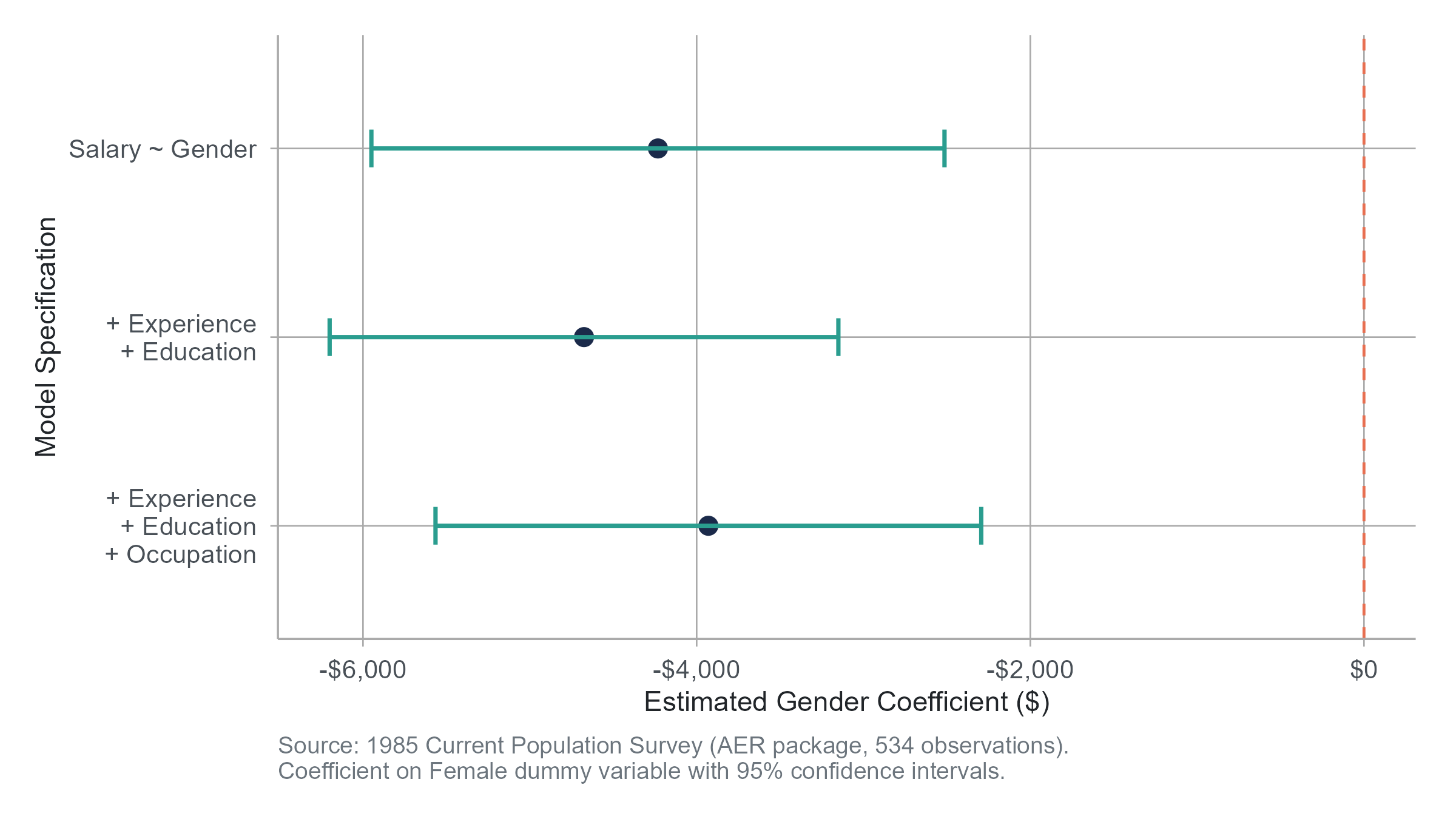
Suppose you regress salary on gender. You find that women earn $4,233 less than men. But you did not include occupation or human capital variables in the model. If women and men tend to work in different occupations (they do), and those occupations pay differently (they do), then the coefficient on gender is picking up two things: the salary difference between men and women within the same occupation, and the salary difference across the occupations that men and women tend to hold. These are very different things, and the coefficient from the simple model mixes them together.

Now suppose you add experience and education to the model. The coefficient on gender actually increases to $4,676. This can happen when the omitted variables work in the opposite direction from what you might expect, in this case, women in the sample having slightly more education on average. Add occupation to the model, and the gender coefficient drops to $3,930 as occupational sorting accounts for some of the gap.

Each time you add a relevant variable, the coefficient on gender changes. This is omitted variable bias at work. The coefficient on any predictor is biased when a relevant variable is left out of the model, as long as the omitted variable is correlated with both the predictor and the outcome.

Figure 11.1: Gender wage coefficient across progressively controlled regression models. Source: 1985 Current Population Survey (534 observations, AER package).

11.9.2 The Formal Condition

Omitted variable bias occurs when two conditions are met simultaneously.

The omitted variable is correlated with the included predictor of interest.
The omitted variable is related to the outcome.

If either condition fails, there is no bias. If an omitted variable affects salary but is completely uncorrelated with gender (say, a random employee ID number that happens to correlate with salary due to some payroll system quirk), leaving it out does not bias the gender coefficient. And if a variable correlates with gender but has no relationship with salary (say, the brand of shampoo the person uses), omitting it does not cause bias either.

11.9.3 The Direction of Bias

You can even predict the direction of the bias. If the omitted variable is positively correlated with both the predictor and the outcome, then leaving it out inflates the coefficient on the predictor (positive bias). If the correlations go in opposite directions, the bias works the other way.

Returning to our wage gap example, experience is positively correlated with salary (more experience, higher pay) and let us suppose it is also positively correlated with being male (men in the sample tend to have more experience). If we leave experience out, the coefficient on the “male” dummy will be too large, overstating the male earnings advantage, because it absorbs some of the experience effect. Adding experience to the model removes that upward bias from the gender coefficient.

11.10 Simpson’s Paradox

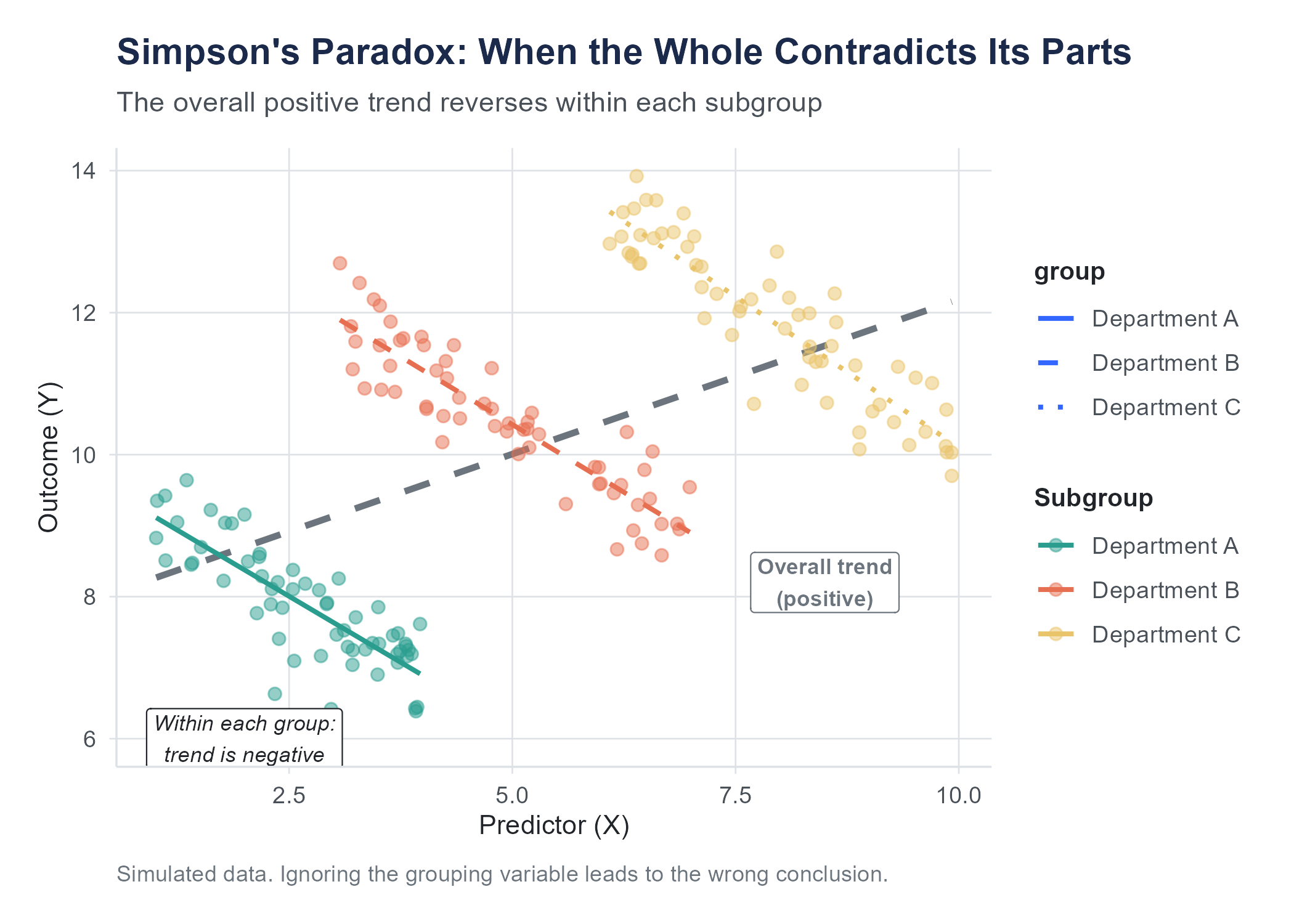
Simpson’s Paradox is a common illustration of how aggregated data can mislead, and it connects directly to the themes of this chapter. It describes a situation where a trend that appears in aggregated data reverses when you look at subgroups. It is not a paradox in the logical sense — it is a consequence of confounding — but it is counterintuitive the first time you encounter it.

11.10.1 The Berkeley Admissions Case

In the fall of 1973, the University of California, Berkeley faced concerns about gender bias in graduate admissions. The aggregate numbers told a stark story: about 44% of male applicants were admitted, compared to only 35% of female applicants. That is a nine-point gap, and it favored men.

But when researchers Peter Bickel, Eugene Hammel, and J. William O’Connell examined admissions at the department level, the picture reversed. In most individual departments, women were admitted at equal or slightly higher rates than men. In some departments, women actually had a higher admission rate.

How is this possible? How can women be disadvantaged overall but advantaged within most departments?

The answer lies in the pattern of applications. Women tended to apply to departments with low overall admission rates, competitive humanities and social science programs that rejected most applicants regardless of gender. Men tended to apply to departments with high overall admission rates, often in engineering and the sciences. When you aggregate across departments, the low admission rates in the departments where women concentrated drag down the overall female admission rate, even though within each department, women did fine.

The confounding variable is department. Department is associated with both gender (men and women applied to different departments) and the outcome (departments had different admission rates). Ignoring department produced a misleading picture. Including it, the equivalent of “controlling for” department in a regression, revealed a very different story.

Figure 11.2: Scatter plot demonstrating Simpson’s Paradox with three subgroups. The overall trend across all data points is positive (dashed line), but within each subgroup the trend is negative (solid lines). Ignoring the grouping variable leads to the opposite conclusion from the one supported by the subgroup-level data.

11.10.2 What Simpson’s Paradox Teaches Us

The lesson is not that you should always look at subgroups. Sometimes the aggregated picture is the right one. The lesson is that the relationship between two variables can change, even reverse, when you account for a third variable. And that means you need to think carefully about which variables to include in your analysis and why. The statistics alone cannot tell you which analysis is “correct.” That requires judgment about the causal structure of the problem, which variables are confounders that should be controlled for, which are mediators that should not be, and which are irrelevant.

This is exactly where the wage gap debate lives. Whether the “raw” gap or the “controlled” gap is the more informative number depends on what question you are trying to answer. Both numbers are correct. They just answer different questions.

11.11 The Ethics of “Controlling Away” Discrimination

Ethics Moment

One consequential misuse of multiple regression is what scholars call “controlling away” discrimination. It works like this.

You start with a raw wage gap between men and women (or between racial groups, or any other comparison). Then you add control variables: occupation, industry, education, experience, hours worked, geographic location. With each variable you add, the gap shrinks. Eventually, someone declares that “after controlling for relevant factors, the gap disappears,” and concludes that there is no discrimination.

The logical error here is subtle but consequential. Many of the variables being “controlled for” are themselves shaped by the very discrimination you are trying to measure. If women are steered away from high-paying occupations by cultural expectations, biased mentoring, hostile workplace cultures, or outright discrimination, then occupation is not an independent factor that explains the gap. It is a mechanism through which discrimination operates. Controlling for it does not eliminate the effect of discrimination. It hides it.

Consider a concrete example. Suppose an employer pays men and women equally within every job title. No discrimination within roles, right? But the employer systematically promotes men to senior roles faster than equally qualified women. If you control for job title in your regression, the gender coefficient goes to zero, and the analysis says there is no pay gap. But the discrimination is real. It just operates through promotion rather than through within-role pay.

This does not mean you should never include occupation or job title in a wage gap analysis. Sometimes the within-occupation gap is exactly the question you want to answer. The point is that the choice of control variables is not a neutral, technical decision. It is a substantive choice that determines what kind of discrimination your analysis can detect and what kind it will miss. An analysis that “controls away” a gap has not demonstrated the absence of discrimination. It has narrowed its gaze to one specific pathway and ignored the others.

When you read or conduct regression analyses involving equity and fairness, ask yourself what the control variables are, whether any of them could be contaminated by the outcome you are studying, and what kinds of disparities the analysis is structurally unable to detect.

This issue extends well beyond gender. In studies of racial disparities in the criminal justice system, researchers sometimes control for “criminal history” when estimating the effect of race on sentencing. But if policing itself is biased, if certain communities are policed more intensively, leading to higher arrest and conviction rates for equivalent behavior, then criminal history is contaminated by the very racial bias the study is trying to measure. Controlling for it masks rather than clarifies the role of race.

The general principle is this. Before you include a variable as a control, ask whether it could be on the causal pathway between the predictor of interest and the outcome. If it is, controlling for it can absorb part or all of the effect you are trying to estimate, leading you to wrongly conclude that no effect exists.

This is not a reason to abandon multiple regression. It is a reason to use it thoughtfully. Regression is a tool, and like any tool, it does what you tell it to, not what you intend. The choice of what to control for is where the intelligence lives.

11.12 The Bias-Variance Trade-Off in Model Building

Building a good multiple regression model requires navigating a fundamental tension. On one side, you want to include enough predictors to capture the real relationships in the data and avoid omitted variable bias. On the other, you want to keep the model parsimonious enough to avoid multicollinearity, overfitting, and uninterpretable results.

This tension is sometimes called the bias-variance trade-off. A model that is too simple (too few predictors) may be biased because it omits important variables. A model that is too complex (too many predictors) may have high variance, with coefficients that jump around wildly from sample to sample and do not generalize well to new data.

There is no formula for resolving this trade-off. It requires judgment. Good practice involves starting with predictors that theory and subject-matter knowledge suggest are important, adding variables incrementally while watching for signs of multicollinearity and overfitting, checking whether adjusted $R^2$ improves with each addition, and resisting the temptation to throw every available variable into the model just because the data exists.

AI Reality Check

Automated feature selection algorithms, built into many statistical and machine learning software packages, promise to solve the model-building problem for you. Stepwise regression, LASSO, elastic net, and similar methods use mathematical criteria to decide which predictors to include. Machine learning pipelines in business settings routinely run through hundreds or thousands of potential predictors and select the combination that optimizes some fit metric.

These tools can be useful, but they can also produce models that are technically optimized and substantively absurd. An automated procedure might find that zip code is the most powerful predictor of loan default, but if the reason zip code predicts default is that it is a proxy for race, the model has baked racial discrimination into its predictions without anyone intending it. A stepwise regression might select predictors that have a spurious correlation with the outcome in your particular sample but no real-world connection to it.

The fundamental problem is that algorithms optimize for a statistical objective (minimizing prediction error, maximizing $R^2$, or similar) without understanding what the variables mean. They do not know that including “number of hospitals within 10 miles” in a model predicting individual health outcomes is capturing geography and socioeconomic status, not some direct effect of hospital proximity. They do not know that selecting “applicant’s first name” as a predictor of job performance is likely encoding racial and ethnic bias.

Use automated feature selection as a tool for exploration, not as a replacement for thinking. After the algorithm suggests a model, ask yourself whether the predictors make substantive sense, whether any of them might be proxies for protected characteristics, and whether the model would hold up with new data from a different context. If you cannot explain why a predictor is in the model, be suspicious.

11.13 Putting It All Together with the Wage Gap

Let us return to where we started and trace through the wage gap analysis step by step, applying everything we have covered.

Step 1, the raw gap. Regress salary on gender (a single dummy variable where Female = 1). You find $b_1 = -4,\!233$. Women earn $4,233 less on average. This is a descriptive fact about the data. It does not tell you why. This model has an $R^2$ of just 0.042, meaning gender alone explains only about 4% of the variation in salaries.

Step 2, adding human capital variables. Add years of experience and years of education to the model. The coefficient on Female changes to $-4,\!676$, while experience contributes $226 per year and education contributes $1,880 per year. The $R^2$ jumps to 0.253. Interestingly, the gender gap actually widens slightly after accounting for experience and education, suggesting that women in this sample have somewhat more education or experience than men on average, and that the raw gap was actually understating the within-group difference. Whether that portion reflects discrimination or other factors is a question regression cannot answer.

Step 3, adding occupation. The coefficient on Female changes to $-3,\!930$, with experience at $206 per year and education at $1,432 per year. The $R^2$ rises to 0.302. Some of the gap is accounted for by the fact that men and women cluster in different occupations, and those occupations pay differently. The question of whether this clustering is itself a product of discrimination is outside the scope of the regression.

Step 4, interpretation. After controlling for experience, education, and occupation, an estimated $3,930 gap remains. This is sometimes called the “unexplained” or “adjusted” gap. Some people interpret it as a lower bound on discrimination (it captures within-category disparities that cannot be attributed to the control variables). Others point out that unmeasured factors could explain even this residual. Both arguments have merit. What neither argument can do is use the regression alone to settle the debate. The regression tells you what the data says under a set of assumptions. Whether those assumptions are reasonable requires thinking about the world, beyond the math.

This is what statistical literacy looks like. Not blind trust in the numbers. Not blanket skepticism either. Just careful, honest engagement with what the analysis can and cannot tell you.

11.14 Assumptions and Diagnostics

Multiple regression, like any statistical method, rests on assumptions. When those assumptions are badly violated, the results can be misleading. Here are the key assumptions and how to check them.

Linearity. The relationship between each predictor and the outcome (after accounting for other predictors) should be approximately linear. Check this by plotting residuals against each predictor. If you see a clear curve, the linearity assumption is violated. Solutions include adding polynomial terms or transforming the variable. A common transformation is the logarithm. When salary data is right-skewed (a few very high earners pulling the distribution), regressing log(salary) on the predictors often produces better-behaved residuals and more interpretable results. In a log-transformed model, coefficients approximate percentage changes rather than dollar changes; each additional year of experience is associated with, say, a 3% increase in salary rather than a flat dollar amount. Log transformations are also useful for predictors. Taking the log of a highly skewed predictor like company revenue or city population can linearize its relationship with the outcome.

Independence of residuals. The residual for one observation should not be correlated with the residual for another. This assumption is often violated with time-series data (today’s stock return is correlated with yesterday’s) or clustered data (students within the same classroom are more similar to each other than to students in other classrooms). Violations require specialized methods like time-series models or multilevel models.

Homoscedasticity. The spread of the residuals should be roughly constant across all levels of the predicted values. If the residuals fan out (getting more spread as $\hat{Y}$ increases), you have heteroscedasticity, and the standard errors of the coefficients may be wrong. A residual-versus-fitted-values plot is the standard diagnostic. If heteroscedasticity is present, you can use robust standard errors or transform the outcome variable.

Normality of residuals. For inference (hypothesis tests and confidence intervals about the coefficients), the residuals should be approximately normally distributed. This is the least important assumption for large samples, because the Central Limit Theorem provides coverage. For small samples, check with a Q-Q plot or a histogram of the residuals. Severe skewness or heavy tails may call for transformations or non-parametric alternatives.

No perfect multicollinearity. As discussed, the predictors should not be perfectly linearly dependent. Check VIF values and correlation matrices (the latter introduced in Chapter 4 as a way to look at all pairwise correlations among numerical variables at once).

No real-world dataset satisfies all these assumptions perfectly. The question is whether violations are severe enough to undermine the conclusions. A mild departure from normality in a sample of 500 is nothing to worry about. Severe heteroscedasticity in a sample of 50 is a real problem. Developing a feel for what matters and what does not is part of the art of regression analysis.

11.15 A Note on Statistical Significance of Individual Predictors

When software reports regression output, each coefficient comes with a standard error, a t-statistic, and a p-value. The p-value tests the null hypothesis that the corresponding population coefficient is zero, that is, that the predictor has no linear relationship with the outcome after accounting for the other predictors.

A small p-value is treated as evidence against the null hypothesis, leading to a conclusion that the predictor has a statistically distinguishable relationship with the outcome. As discussed in Chapter 8, the conventional 0.05 threshold is exactly that — a convention — and a p-value of 0.04 is not categorically different from one of 0.06. A large p-value means you cannot rule out the possibility that the predictor’s apparent relationship is due to sampling variability.

But remember from Chapter 8 that statistical significance is not the same as practical importance. A coefficient of $50 on some predictor might be statistically significant with a large enough sample, but $50 per unit change might be meaningless in context. Conversely, a coefficient of $5,000 might not reach statistical significance in a small sample, even though a $5,000 difference would be quite meaningful if real.

Report coefficients and their confidence intervals alongside p-values. The coefficient tells you how big the estimated effect is. The confidence interval tells you how uncertain you are. The p-value tells you whether the data are consistent with no effect at all. All three pieces of information are needed for a complete picture.

When the Outcome Is Yes or No

Everything in this chapter assumes the outcome variable is numerical: salary, test scores, blood pressure. But many important outcomes in business and social science are binary: Did the customer buy or not? Did the patient survive or not? Did the loan default or not? Was the applicant hired or not?

Linear regression is not appropriate for binary outcomes. If you try to predict a 0/1 variable with ordinary least squares, the model can produce predicted values below 0 or above 1, which make no sense as probabilities. The solution is logistic regression, which models the probability of the outcome occurring rather than the outcome itself. Instead of a straight line, it fits an S-shaped curve (the logistic function) that keeps predicted probabilities between 0 and 1.

Logistic regression is beyond the scope of this book, but it uses the same logic of multiple predictors, coefficients, and “holding other variables constant” that you learned here. If your next course or job requires you to model binary outcomes, you already have the conceptual foundation. The leap from linear to logistic is smaller than it looks.

11.16 Looking Ahead

This chapter has taken you from simple regression, one predictor and one outcome, to the far richer world of multiple regression, where several predictors work together (and sometimes against each other) to explain variation in an outcome. You have learned what “controlling for” really means, why it can go wrong, and how to think critically about which variables belong in a model and which do not. With this foundation, you now have the core toolkit of applied statistical analysis: description, probability, inference, and modeling. The final chapter steps back from the mechanics and looks forward. What lies beyond introductory statistics? Where do these methods lead? And what responsibilities come with the ability to analyze data? Those are the questions we close with.

11.17 Further Reading and References

The following works are cited in this chapter or provide valuable additional context for the ideas covered here.

On the gender wage gap: Blau, F. D., & Kahn, L. M. (2017). The gender wage gap: Extent, trends, and explanations. Journal of Economic Literature, 55(3), 789–865. (A comprehensive review of the wage gap literature, including the role of occupation, human capital, and discrimination, directly relevant to this chapter’s opening example.)

On the Berkeley admissions case: Bickel, P. J., Hammel, E. A., & O’Connell, J. W. (1975). Sex bias in graduate admissions: Data from Berkeley. Science, 187(4175), 398–404. (The original analysis that uncovered Simpson’s Paradox in Berkeley’s graduate admissions, one of the most cited examples of how aggregated data can mislead.)

On causal inference with regression: Angrist, J. D., & Pischke, J.-S. (2014). Mastering ’metrics: The path from cause to effect. Princeton University Press. (An accessible introduction to regression as a tool for causal inference, with a clear treatment of omitted variable bias and the conditions under which regression coefficients can be interpreted causally.)

Cunningham, S. (2021). Causal inference: The mixtape. Yale University Press. (Available free online, covers similar ground with more examples and a conversational style. An excellent next step if this chapter’s treatment of causality left you wanting more.)

On the ethics of “controlling away” discrimination: Goldin, C. (2014). A grand gender convergence: Its last chapter. American Economic Review, 104(4), 1091–1119. (A comprehensive analysis showing that the remaining gender wage gap is driven less by occupation-level sorting and more by within-occupation differences in how work is structured and rewarded, challenging the assumption that controlling for occupation eliminates discrimination.)

For further reading on multiple regression: Gelman, A., Hill, J., & Vehtari, A. (2020). Regression and other stories. Cambridge University Press. (A modern treatment of regression that emphasizes interpretation, causal reasoning, and practical diagnostics, building naturally on the concepts introduced in this chapter.)

11.18 Key Terms

Multiple regression: A statistical model that relates an outcome variable to two or more predictor variables. The general form is $Y = b_0 + b_1 X_1 + b_2 X_2 + \cdots + b_k X_k + e$.
Regression coefficient ($b_j$): The estimated change in the outcome associated with a one-unit increase in predictor $X_j$, holding all other predictors in the model constant.
Dummy variable (indicator variable): A variable that takes the value 1 if a condition is true and 0 if it is false, used to include categorical predictors in a regression model.
Reference category: The category of a categorical variable that is coded as 0 on all dummy variables. Coefficients on the dummy variables represent comparisons to this baseline group.
R-squared ($R^2$): The proportion of the variance in the outcome that is explained by the regression model. Ranges from 0 to 1, but always increases (or stays the same) when a predictor is added.
Adjusted R-squared ($R^2_{adj}$): A modified version of $R^2$ that includes a penalty for the number of predictors, making it more appropriate for comparing models of different sizes.
Multicollinearity: A condition in which two or more predictor variables in a regression model are highly correlated with each other, making it difficult to separate their individual effects on the outcome.
Variance Inflation Factor (VIF): A diagnostic measure for multicollinearity. VIF values above 5 or 10 indicate concerning levels of correlation among predictors.
Omitted variable bias: The bias in a regression coefficient that occurs when a relevant variable is left out of the model and that variable is correlated with both the included predictor and the outcome.
Confounder (confounding variable): A variable that influences both the explanatory variable and the response variable, creating a misleading association between them if not accounted for.
Mediator: A variable that lies on the causal pathway between the predictor and the outcome. Controlling for a mediator removes part of the predictor’s effect, which may or may not be desirable.
Simpson’s Paradox: A phenomenon in which a trend that appears in aggregated data reverses or disappears when the data is separated into subgroups. It arises from confounding.
Heteroscedasticity: A condition in which the spread of the residuals varies across levels of the predicted values, violating one of the assumptions of ordinary least squares regression.
Homoscedasticity: The assumption that the variance of the residuals is constant across all levels of the predicted values. The opposite of heteroscedasticity.
Interaction effect: A situation in which the relationship between one predictor and the outcome depends on the value of another predictor.
Interaction term: A variable created by multiplying two predictors together, included in the model to capture an interaction effect.
Logistic regression: A regression method for binary outcomes (yes/no, 0/1) that models the probability of the outcome using an S-shaped curve. Beyond the scope of this book but uses the same logic of multiple predictors and “holding constant” developed here.
Controlling for (a variable): Including a variable in a regression model so that the coefficients on other predictors represent relationships that hold after accounting for that variable. Only as good as the model’s assumptions and the variables included.
Bias-variance trade-off: The tension between using a simple model (which may be biased due to omitted variables) and a complex model (which may have high variance and overfit the data).

11.19 Exercises

11.19.1 Check Your Understanding

Write out the general form of a multiple regression model with three predictors. Label each component and explain what it represents.
In a regression of salary on experience and education, the coefficient on experience is $1,850. A student says, “Each year of experience increases your salary by $1,850.” What is missing from this interpretation? Rewrite it more carefully.
Explain why you need $k - 1$ dummy variables to represent a categorical variable with $k$ categories. What happens if you include all $k$ dummy variables instead?
A researcher fits two models. Model A has three predictors and an $R^2$ of 0.42. Model B has ten predictors and an $R^2$ of 0.47. The researcher concludes that Model B is better because it explains more variance. What is wrong with this reasoning? What measure should the researcher use instead?
Define multicollinearity in your own words. Give an example of two predictor variables that you would expect to be highly collinear if both were included in a regression model predicting household spending.
A regression model has a VIF of 8.3 for one of its predictors. What does this tell you? What are your options for addressing the problem?
Explain the difference between a confounder and a mediator. Why does the distinction matter for deciding which variables to include in a regression model?
State the two conditions that must be met for omitted variable bias to occur. For each condition, explain what happens if that condition is not met (that is, why there is no bias in that case).
Describe Simpson’s Paradox in your own words. Give an example (different from the Berkeley admissions case discussed in the chapter) where aggregated data might reverse a trend visible in subgroups.
A news headline reads, “After controlling for education, experience, and occupation, the racial wage gap in tech is only 1.2%.” A reader concludes that there is very little discrimination in tech. What important question should the reader ask before accepting this conclusion?

11.19.2 Apply It

(See Appendix B for complete variable descriptions for all datasets used in these exercises.)

Use the wage-gap.csv dataset for the following problems. This dataset contains real data from the 1985 Current Population Survey (CPS), sourced from the AER R package. Note that salaries are in 1985 dollars. The dataset contains 534 observations with the following variables.

Variable	Description
`employee_id`	Unique identifier for each worker
`salary`	Annual salary in dollars (1985 dollars)
`gender`	“Male” or “Female”
`years_experience`	Years of work experience
`education_years`	Years of formal education
`occupation`	Occupation category (six levels: “Worker,” “Technical,” “Services,” “Office,” “Sales,” “Management”)
`region`	Geographic region (“South” or “Other”)
`union_member`	Whether the worker is a union member
`married`	Marital status
`ethnicity`	Worker’s ethnicity

Fit a simple regression model predicting salary from gender alone (with “Male” as the reference category). Report the intercept and the coefficient on Female. Interpret both values in context. What does this model tell you about the raw wage gap in these data?
Now fit a multiple regression model predicting salary from gender, years_experience, and education_years. Report all coefficients. How does the coefficient on Female change compared to the simple regression in Problem 1? What does this change suggest about the role of experience and education in explaining the raw wage gap?
Create dummy variables for occupation (using “Manufacturing” as the reference category) and add them to the model from Problem 2. Report the coefficient on Female and the coefficients on each occupation dummy. Which occupation has the highest estimated salary relative to Manufacturing, holding other variables constant? How did adding occupation affect the gender gap coefficient?
Add region to the model (using “Other” as the reference category). Report the full regression equation with all coefficients. How does the estimated salary in the South compare to the Other region? Is the difference statistically significant at the 0.05 level?
Add union_member, married, and ethnicity to the model. Report the new coefficient on Female and the adjusted $R^2$ for the model with and without these additional variables. Did the addition of these variables improve the model according to adjusted $R^2$? How did they affect the gender gap coefficient?
For your full model (with all predictors), calculate and report the VIF for each predictor. Are any predictors showing signs of concerning multicollinearity? If so, which ones and what would you recommend?
Compare the $R^2$ and adjusted $R^2$ for the following three models: (a) salary on gender alone, (b) salary on gender, years_experience, and education_years, (c) the full model with all predictors. For each step, note whether adjusted $R^2$ increased and by how much. What do these comparisons tell you about the relative importance of different groups of predictors?
Using your full model, compute the predicted salary for a female worker with 10 years of experience, 16 years of education, in the Technical occupation in the South, who is not a union member, is married, and of Hispanic ethnicity. Then compute the predicted salary for a male worker with identical characteristics. What is the difference? Does this match the coefficient on Female? Explain why or why not.
Fit two models: one predicting salary from years_experience alone, and another predicting salary from both years_experience and education_years. Compare the coefficient on years_experience in the two models. Did it increase, decrease, or stay about the same? Using the concept of omitted variable bias, explain why the coefficient changed in the direction it did. (Hint: think about the correlation between experience and education, and the relationship between education and salary.)
Create a residual plot for your full model (residuals on the vertical axis, predicted values on the horizontal axis). Does the plot suggest any violations of the assumptions of linear regression? Specifically, comment on whether the residuals appear to have constant variance (homoscedasticity) and whether there are any obvious patterns suggesting non-linearity.
Interaction effect. Fit a model predicting salary from years_experience, gender, and the interaction years_experience × gender. In R, lm(salary ~ years_experience * gender, data = ...) includes both main effects and the interaction in one shot. Report the coefficients on years_experience, genderFemale (assuming Male is the reference), and the interaction term years_experience:genderFemale. Interpret each coefficient. According to this model, is the dollar return to an additional year of experience the same for men and women, or different — and by how much? Sketch (or actually plot) the two predicted regression lines, one for men and one for women, on the same axes. Why is this different information from a model that just adds gender as a control without the interaction term?

11.19.3 Think Deeper

Return to the wage gap analysis from this chapter. Suppose you are advising a policymaker who asks you, “What is the gender wage gap?” How would you explain that there is not a single answer to this question, but rather multiple answers depending on what you control for and why? What question does the raw gap answer? What question does the fully controlled gap answer? Why might a policymaker want both numbers?
A company analyzes its pay data and finds that after controlling for job title, department, and years of service, there is no statistically significant pay gap between male and female employees. The CEO announces that the analysis proves the company has pay equity. Write a memo to the CEO explaining why this conclusion may be premature. Be specific about which forms of potential discrimination the analysis can detect and which it cannot.
A health insurance company builds a regression model to predict healthcare costs. The model includes age, BMI, smoking status, number of chronic conditions, and zip code. A data scientist notices that zip code is one of the strongest predictors. The company plans to use the model to set premium rates. Discuss the ethical implications. What might zip code be capturing that makes it such a powerful predictor? What are the potential consequences of using zip code in rate-setting? Should the company remove zip code from the model, even if doing so makes the predictions less accurate?
A researcher studying the effect of class size on student test scores obtains data from 500 schools. The researcher regresses average test scores on average class size and finds a negative relationship: smaller classes are associated with higher scores. The researcher concludes that reducing class size improves learning. A colleague points out that wealthier school districts tend to have smaller classes and also tend to have students who score higher for many other reasons (parental involvement, private tutoring, better facilities). The colleague says the result is driven by omitted variable bias. The researcher responds by adding average household income as a control variable. Is this sufficient to address the concern? What other variables might still be missing? Is there a study design that would more convincingly establish a causal effect of class size?
Consider a criminal justice dataset where researchers examine the relationship between race and sentencing length. They control for “severity of the offense” and “prior criminal record.” After adding these controls, the racial gap in sentencing shrinks considerably. A commentator writes, “Once you account for the nature of the crime and the defendant’s history, race plays almost no role.” Critically evaluate this claim. Under what circumstances could “severity of the offense” and “prior criminal record” themselves be influenced by racial bias in the justice system? What does controlling for them potentially mask?
In the Berkeley admissions example discussed in this chapter, the aggregated data showed women admitted at lower rates than men, but department-level data showed women admitted at equal or higher rates. Now consider a hypothetical in the opposite direction. Suppose aggregated data shows equal admission rates for men and women, but at the department level, men are admitted at higher rates in every single department. Construct a numerical example with at least three departments showing how this could happen. (Hint: think about which departments have high admission rates and which have low ones, and how men and women distribute across them.) What lesson does this reinforce about the importance of disaggregating data?