Chapter 7: Confidence Intervals

Overview

A confidence interval quantifies our uncertainty about a population parameter. Instead of reporting a single estimate, we provide a range of plausible values — and state how confident we are that the range captures the truth. In this walkthrough, we build confidence intervals by hand, verify them with t.test(), and run a simulation that reveals what “95% confidence” actually means. This walkthrough accompanies Chapter 7 of Margin of Error.

Setup

# Loads tidyverse, book color palette, and theme_moe()
# Download _common.R from the Datasets page if running locally
source("_common.R")

Building a Confidence Interval by Hand

Suppose we draw a sample of n = 36 observations and find a sample mean of 72 with a standard deviation of 12. The 95% CI for the population mean is:

\[ \bar{x} \pm t^* \times \frac{s}{\sqrt{n}} \]

xbar <- 72
s <- 12
n <- 36

t_star <- qt(0.975, df = n - 1)
margin_of_error <- t_star * s / sqrt(n)

lower <- xbar - margin_of_error
upper <- xbar + margin_of_error

cat("t* (df =", n - 1, "):", round(t_star, 4), "\n")

t* (df = 35 ): 2.0301

cat("Margin of error:", round(margin_of_error, 2), "\n")

Margin of error: 4.06

cat("95% CI: [", round(lower, 2), ",", round(upper, 2), "]\n")

95% CI: [ 67.94 , 76.06 ]

Using `t.test()` to Get a CI

In practice, you let R do the arithmetic. The t.test() function returns a confidence interval directly.

set.seed(42)
sample_data <- rnorm(36, mean = 72, sd = 12)

result <- t.test(sample_data, conf.level = 0.95)
result$conf.int

[1] 67.90930 77.71205
attr(,"conf.level")
[1] 0.95

cat("Sample mean:", round(result$estimate, 2), "\n")

Sample mean: 72.81

cat("95% CI: [", round(result$conf.int[1], 2), ",",
    round(result$conf.int[2], 2), "]\n")

95% CI: [ 67.91 , 77.71 ]

Confidence Interval for a Proportion

For a proportion, the formula uses the normal approximation:

\[ \hat{p} \pm z^* \times \sqrt{\frac{\hat{p}(1 - \hat{p})}{n}} \]

Suppose in a poll of 400 voters, 220 support a ballot measure.

p_hat <- 220 / 400
n_prop <- 400
z_star <- qnorm(0.975)

me_prop <- z_star * sqrt(p_hat * (1 - p_hat) / n_prop)

cat("Sample proportion:", p_hat, "\n")

Sample proportion: 0.55

cat("Margin of error:", round(me_prop, 4), "\n")

Margin of error: 0.0488

cat("95% CI: [", round(p_hat - me_prop, 4), ",",
    round(p_hat + me_prop, 4), "]\n")

95% CI: [ 0.5012 , 0.5988 ]

We can also use prop.test():

prop.test(220, 400, conf.level = 0.95, correct = FALSE)$conf.int

[1] 0.5010010 0.5980478
attr(,"conf.level")
[1] 0.95

Coverage Simulation: What Does “95% Confidence” Mean?

If we repeated our study many times, about 95% of the resulting intervals should capture the true population mean. Let’s verify by simulation: draw 100 samples from a known population, compute a CI for each, and see how many capture the truth.

set.seed(42)
true_mean <- 50
true_sd <- 10
n_sim <- 30
n_intervals <- 100

sim_results <- map_dfr(1:n_intervals, function(i) {
  samp <- rnorm(n_sim, mean = true_mean, sd = true_sd)
  test <- t.test(samp, conf.level = 0.95)
  tibble(
    interval = i,
    lower = test$conf.int[1],
    upper = test$conf.int[2],
    captures = lower <= true_mean & upper >= true_mean
  )
})

coverage <- mean(sim_results$captures)
cat("Intervals that capture the true mean:", sum(sim_results$captures),
    "out of", n_intervals, "\n")

Intervals that capture the true mean: 95 out of 100

cat("Coverage rate:", coverage * 100, "%\n")

Coverage rate: 95 %

ggplot(sim_results, aes(y = interval)) +
  geom_segment(aes(x = lower, xend = upper, yend = interval,
                   color = captures), linewidth = 0.5) +
  geom_vline(xintercept = true_mean, linetype = "dashed",
             color = moe_colors$navy, linewidth = 0.8) +
  scale_color_manual(
    values = c("TRUE" = moe_colors$teal, "FALSE" = moe_colors$coral),
    labels = c("TRUE" = "Captures true mean", "FALSE" = "Misses")
  ) +
  labs(
    title = "100 Confidence Intervals from Repeated Sampling",
    subtitle = paste0("Coverage: ", sum(sim_results$captures),
                      " out of 100 capture the true mean (dashed line)"),
    x = "Value",
    y = "Interval number",
    color = NULL
  ) +
  theme_moe()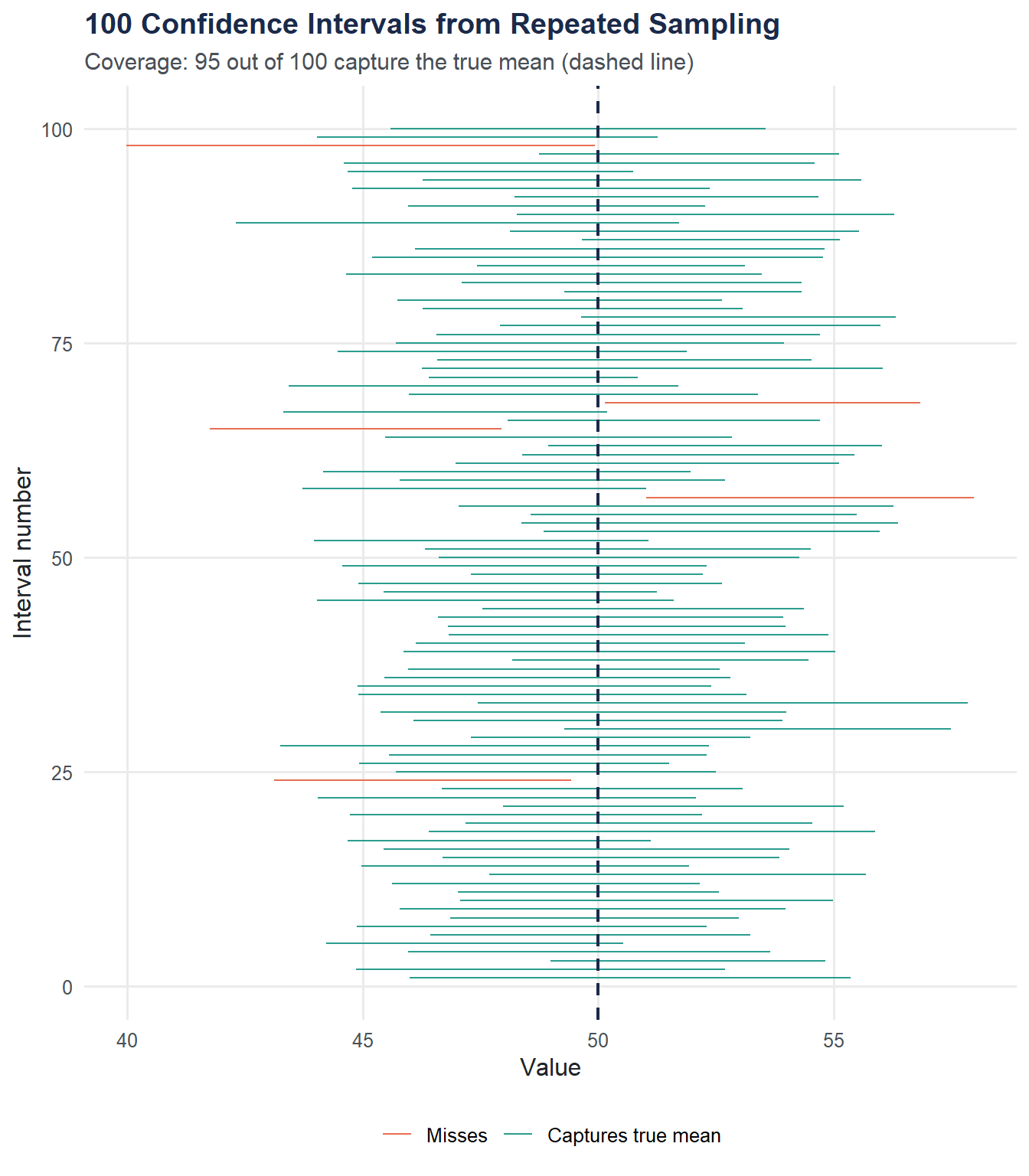

Figure 1: 100 confidence intervals: green captures the true mean, coral misses

Most intervals contain the true mean, but a few miss. That is exactly what “95% confidence” means: not every interval is correct, but the procedure works about 95% of the time in the long run.

Effect of Sample Size on CI Width

Larger samples give more precise estimates. The margin of error shrinks by a factor of \(1/\sqrt{n}\).

set.seed(42)
sample_sizes <- c(10, 30, 100, 500)

size_results <- map_dfr(sample_sizes, function(n_size) {
  samp <- rnorm(n_size, mean = 50, sd = 10)
  test <- t.test(samp, conf.level = 0.95)
  tibble(
    n = paste("n =", n_size),
    lower = test$conf.int[1],
    upper = test$conf.int[2],
    width = upper - lower,
    mean = test$estimate
  )
})

size_results$n <- factor(size_results$n,
                         levels = paste("n =", sample_sizes))

ggplot(size_results, aes(y = n)) +
  geom_segment(aes(x = lower, xend = upper, yend = n),
               linewidth = 1.5, color = moe_colors$teal) +
  geom_point(aes(x = mean), size = 3, color = moe_colors$navy) +
  geom_vline(xintercept = 50, linetype = "dashed", color = moe_colors$coral) +
  labs(
    title = "CI Width Shrinks with Larger Samples",
    subtitle = "Dashed line = true population mean (50)",
    x = "Value",
    y = NULL
  ) +
  theme_moe()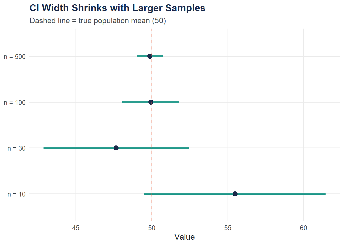

Figure 2: Confidence interval width decreases as sample size increases

Effect of Confidence Level

Higher confidence requires a wider interval. Compare 90%, 95%, and 99% intervals from the same sample.

set.seed(42)
samp <- rnorm(50, mean = 50, sd = 10)

conf_levels <- c(0.90, 0.95, 0.99)

level_results <- map_dfr(conf_levels, function(cl) {
  test <- t.test(samp, conf.level = cl)
  tibble(
    level = paste0(cl * 100, "%"),
    lower = test$conf.int[1],
    upper = test$conf.int[2],
    width = upper - lower,
    mean = test$estimate
  )
})

level_results$level <- factor(level_results$level,
                              levels = c("90%", "95%", "99%"))

ggplot(level_results, aes(y = level)) +
  geom_segment(aes(x = lower, xend = upper, yend = level),
               linewidth = 1.5, color = moe_colors$navy) +
  geom_point(aes(x = mean), size = 3, color = moe_colors$coral) +
  geom_vline(xintercept = 50, linetype = "dashed", color = moe_colors$slate) +
  labs(
    title = "Confidence Level vs. Interval Width",
    subtitle = "More confidence = wider interval (same data, n = 50)",
    x = "Value",
    y = "Confidence Level"
  ) +
  theme_moe()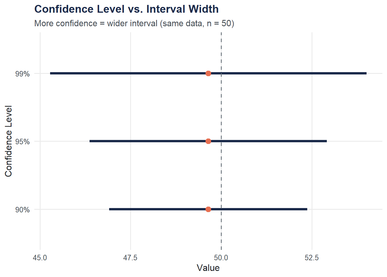

Figure 3: Higher confidence levels produce wider intervals

Try It Yourself

Sample size and margin of error. If you increase the sample size from 30 to 120, by what factor does the margin of error decrease? Compute the ratio \(\sqrt{30} / \sqrt{120}\) and verify it matches the ratio of the two margins of error from t.test().
Coverage at 90% confidence. Re-run the coverage simulation above but change conf.level to 0.90. Do roughly 90 out of 100 intervals capture the true mean?