# Loads tidyverse, book color palette, and theme_moe()
# Download _common.R from the Datasets page if running locally
source("_common.R")Chapter 9: Comparing Groups
Overview
When you have more than two groups, ANOVA lets you test whether their means differ in a statistically meaningful way. In this walkthrough, we extend the resume study analysis from earlier chapters to compare callback rates and experience levels across multiple categories. This walkthrough accompanies Chapter 9 of Margin of Error.
Setup
Load and Explore the Data
The dataset contains 4,870 fictitious resumes sent in response to job postings. Each row records whether the resume received a callback, along with attributes like name type, gender, quality, experience, and education level.
resumes <- read_csv("data/resume-callbacks.csv")Rows: 4870 Columns: 7
── Column specification ────────────────────────────────────────────────────────
Delimiter: ","
chr (5): name_type, gender, resume_quality, education, callback
dbl (2): resume_id, years_experience
ℹ Use `spec()` to retrieve the full column specification for this data.
ℹ Specify the column types or set `show_col_types = FALSE` to quiet this message.glimpse(resumes)Rows: 4,870
Columns: 7
$ resume_id <dbl> 1, 2, 3, 4, 5, 6, 7, 8, 9, 10, 11, 12, 13, 14, 15, 16…
$ name_type <chr> "White-sounding", "White-sounding", "Black-sounding",…
$ gender <chr> "Female", "Female", "Female", "Female", "Female", "Ma…
$ resume_quality <chr> "Low", "High", "Low", "High", "High", "Low", "High", …
$ years_experience <dbl> 6, 6, 6, 6, 22, 6, 5, 21, 3, 6, 8, 8, 4, 4, 5, 4, 5, …
$ education <chr> "Bachelor", "High School", "Bachelor", "High School",…
$ callback <chr> "No", "No", "No", "No", "No", "No", "No", "No", "No",…Before jumping into ANOVA, let’s get a feel for callback rates across the key grouping variables.
resumes |>
  group_by(resume_quality, education) |>
  summarize(
    n = n(),
    callback_rate = round(mean(callback) * 100, 1),
    .groups = "drop"
  )
Warning: There were 4 warnings in `summarize()`.
The first warning was:
ℹ In argument: `callback_rate = round(mean(callback) * 100, 1)`.
ℹ In group 1: `resume_quality = "High"` `education = "Bachelor"`.
Caused by warning in `mean.default()`:
! argument is not numeric or logical: returning NA
ℹ Run `dplyr::last_dplyr_warnings()` to see the 3 remaining warnings.# A tibble: 4 × 4
resume_quality education n callback_rate
<chr> <chr> <int> <dbl>
1 High Bachelor 1771 NA
2 High High School 675 NA
3 Low Bachelor 1733 NA
4 Low High School 691 NAOne-Way ANOVA: Experience by Education Level
Does years of experience differ by education level? A one-way ANOVA tests whether the group means are equal.
aov_model <- aov(years_experience ~ education, data = resumes)
summary(aov_model)
Df Sum Sq Mean Sq F value Pr(>F)
education 1 69 68.56 2.695 0.101
Residuals 4868 123838 25.44 The F-statistic measures how much the group means vary relative to within-group variation. A large F (with a small p-value) suggests that at least one education group has a meaningfully different average experience level.
Tukey HSD: Pairwise Comparisons
ANOVA tells us something differs, but not what. Tukey’s Honest Significant Difference test compares every pair of groups while controlling for multiple comparisons.
tukey_result <- TukeyHSD(aov_model)
tukey_result
Tukey multiple comparisons of means
95% family-wise confidence level
Fit: aov(formula = years_experience ~ education, data = resumes)
$education
diff lwr upr p adj
High School-Bachelor 0.2641073 -0.05129538 0.5795099 0.1007346Look for confidence intervals that do not cross zero — those pairs have statistically significant differences.
Effect Size: Eta-Squared
Statistical significance does not tell us how large the effect is. Eta-squared gives the proportion of total variance explained by the grouping variable.
aov_summary <- summary(aov_model)[[1]]
ss_between <- aov_summary[["Sum Sq"]][1]
ss_total <- sum(aov_summary[["Sum Sq"]])
eta_sq <- ss_between / ss_total

cat("Eta-squared:", round(eta_sq, 4), "\n")
Eta-squared: 6e-04 cat("Interpretation:", round(eta_sq * 100, 1), "% of variance in experience is explained by education level\n")Interpretation: 0.1 % of variance in experience is explained by education levelGuidelines: eta-squared of 0.01 is small, 0.06 is medium, and 0.14 or above is large.
Diagnostic Plots
ANOVA assumes normality of residuals and equal variances across groups. The built-in diagnostic plots help you check these assumptions.
par(mfrow = c(2, 2))
plot(aov_model)
par(mfrow = c(1, 1))
- Residuals vs Fitted: look for a random scatter (no pattern means the equal-variance assumption holds).
- Normal Q-Q: points should fall roughly on the diagonal line.
- Scale-Location: a flat trend line supports equal variance.
- Residuals vs Leverage: flags influential observations.
Visualization: Experience by Education
A boxplot with jittered points shows both the distribution shape and individual data points.
ggplot(resumes, aes(x = education, y = years_experience, fill = education)) +
  geom_boxplot(alpha = 0.6, outlier.shape = NA) +
  geom_jitter(width = 0.2, alpha = 0.15, size = 0.8, color = moe_colors$navy) +
  scale_fill_moe() +
  labs(
    title = "Years of Experience by Education Level",
    subtitle = "Boxplots with individual observations (jittered)",
    x = "Education Level",
    y = "Years of Experience"
  ) +
  theme_moe() +
  theme(legend.position = "none")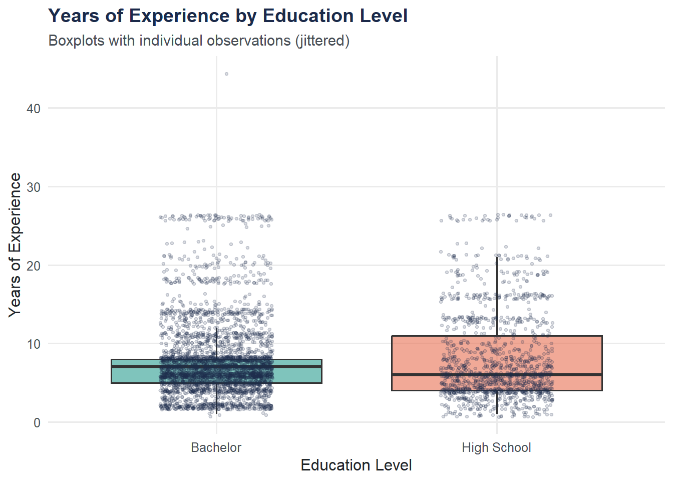
Try It Yourself
Two-way ANOVA. Run an ANOVA comparing
years_experienceacross all combinations ofname_typeandresume_quality. Use the formulaaov(years_experience ~ name_type * resume_quality, data = resumes). Examine the summary — is there a significant interaction between name type and resume quality?QQ plot of residuals. Extract residuals from your two-way ANOVA model with
resid()and create a QQ plot usingqqnorm()andqqline(). Do the residuals appear approximately normal?