# Loads tidyverse, book color palette, and theme_moe()
# Download _common.R from the Datasets page if running locally
source("_common.R")Chapter 12: What Comes Next
Overview
The statistical foundations you have built throughout this book — summarizing data, testing hypotheses, fitting regression models — are a launching pad, not a destination. This brief walkthrough previews several directions your skills can take you. Each section offers a taste of a broader field, with just enough code to spark curiosity. This walkthrough accompanies Chapter 12 of Margin of Error.
Setup
Time Series Analysis
Time series data have a natural ordering — measurements collected over time. Trends, seasonality, and cycles become visible when you plot them.
air_df <- data.frame(
  date = seq(as.Date("1949-01-01"), by = "month", length.out = length(AirPassengers)),
  passengers = as.numeric(AirPassengers)
)

ggplot(air_df, aes(x = date, y = passengers)) +
  geom_line(color = moe_colors$teal, linewidth = 0.8) +
  labs(
    title = "Monthly Airline Passengers",
    subtitle = "A classic time series with trend and seasonality",
    x = "Date",
    y = "Passengers (thousands)"
  ) +
  theme_moe()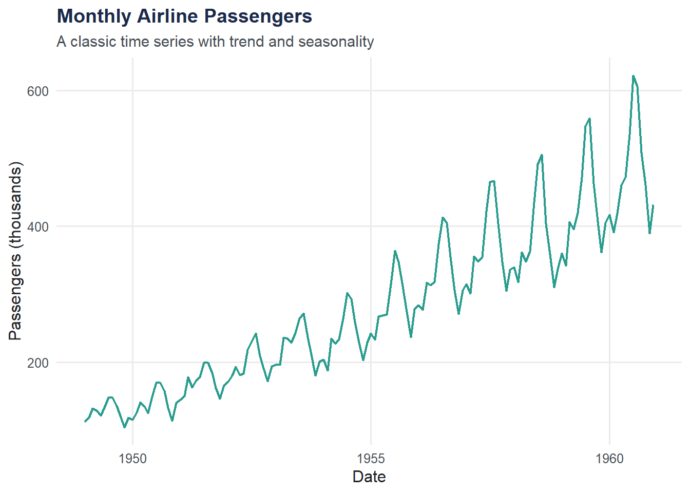
Two features stand out: an upward trend (air travel grew steadily) and seasonality (peaks every summer). Time series methods like ARIMA, exponential smoothing, and decomposition are designed to model exactly these patterns. The forecast and tsibble packages in R provide a full toolkit.
Machine Learning: Classification
Machine learning shifts the goal from explanation to prediction. Instead of interpreting coefficients, we ask: can the model accurately predict an outcome it has never seen? Here we use the resume callback data to build a simple logistic regression classifier.
resumes <- read_csv("data/resume-callbacks.csv") |>
  mutate(callback = ifelse(callback == "Yes", 1, 0))
Rows: 4870 Columns: 7
── Column specification ────────────────────────────────────────────────────────
Delimiter: ","
chr (5): name_type, gender, resume_quality, education, callback
dbl (2): resume_id, years_experience
ℹ Use `spec()` to retrieve the full column specification for this data.
ℹ Specify the column types or set `show_col_types = FALSE` to quiet this message.# Split into training (70%) and test (30%) sets
set.seed(42)
train_index <- sample(seq_len(nrow(resumes)), size = 0.7 * nrow(resumes))
train <- resumes[train_index, ]
test <- resumes[-train_index, ]
cat("Training set:", nrow(train), "rows\n")Training set: 3409 rowscat("Test set:", nrow(test), "rows\n")Test set: 1461 rowsml_model <- glm(callback ~ resume_quality + years_experience,
data = train, family = "binomial")
summary(ml_model)
Call:
glm(formula = callback ~ resume_quality + years_experience, family = "binomial",
    data = train)

Coefficients:
                  Estimate Std. Error z value Pr(>|z|)
(Intercept)       -2.65987    0.13248 -20.078  < 2e-16 ***
resume_qualityLow -0.20240    0.12694  -1.594  0.11083
years_experience   0.04031    0.01094   3.684  0.00023 ***
---
Signif. codes:  0 '***' 0.001 '**' 0.01 '*' 0.05 '.' 0.1 ' ' 1

(Dispersion parameter for binomial family taken to be 1)

    Null deviance: 1931.2  on 3408  degrees of freedom
Residual deviance: 1914.7  on 3406  degrees of freedom
AIC: 1920.7

Number of Fisher Scoring iterations: 5test$predicted_prob <- predict(ml_model, newdata = test, type = "response")
test$predicted_class <- ifelse(test$predicted_prob > 0.5, 1, 0)
accuracy <- mean(test$predicted_class == test$callback)
cat("Test set accuracy:", round(accuracy * 100, 1), "%\n")Test set accuracy: 92.3 %This is the simplest possible version. Real machine learning pipelines involve cross-validation, feature engineering, model comparison (random forests, gradient boosting, neural networks), and careful evaluation with metrics beyond accuracy. The tidymodels framework in R provides a unified interface for all of this.
Bayesian Statistics: Updating Beliefs with Data
Classical (frequentist) statistics asks: “How likely is this data, given a hypothesis?” Bayesian statistics flips the question: “How likely is the hypothesis, given the data?” It starts with a prior belief and updates it to a posterior using observed evidence.
Suppose we want to estimate the true callback rate from the resume study. Before looking at data, we might assume it could be anywhere between 0% and 100% — a flat (uninformative) prior: Beta(1, 1).
resumes <- read_csv("data/resume-callbacks.csv") |>
  mutate(callback = ifelse(callback == "Yes", 1, 0))
Rows: 4870 Columns: 7
── Column specification ────────────────────────────────────────────────────────
Delimiter: ","
chr (5): name_type, gender, resume_quality, education, callback
dbl (2): resume_id, years_experience
ℹ Use `spec()` to retrieve the full column specification for this data.
ℹ Specify the column types or set `show_col_types = FALSE` to quiet this message.successes <- sum(resumes$callback)
failures <- nrow(resumes) - successes
x <- seq(0, 0.20, length.out = 500)
prior <- dbeta(x, 1, 1)
posterior <- dbeta(x, 1 + successes, 1 + failures)
bayes_df <- data.frame(
x = rep(x, 2),
density = c(prior, posterior),
distribution = rep(c("Prior: Beta(1,1)", "Posterior"), each = length(x))
)
ggplot(bayes_df, aes(x = x, y = density, color = distribution)) +
geom_line(linewidth = 1.2) +
scale_color_manual(values = c(moe_colors$slate, moe_colors$coral)) +
labs(
title = "Bayesian Updating",
subtitle = "The flat prior becomes a sharp posterior after 4,870 observations",
x = "Callback Rate",
y = "Density",
color = NULL
) +
theme_moe()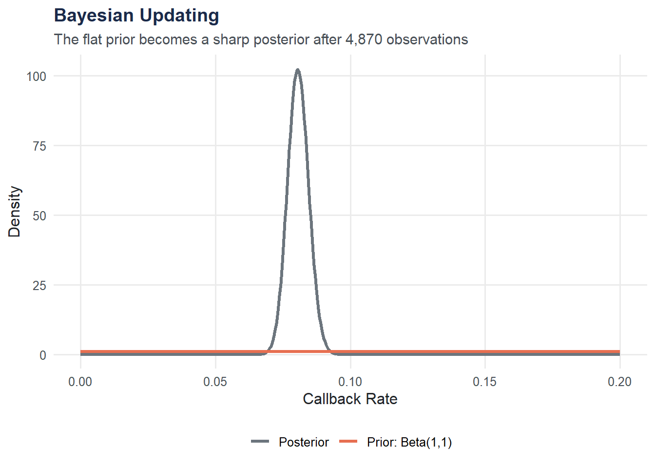
With nearly 5,000 observations, the posterior is tightly concentrated around the observed callback rate. The prior barely matters here — but with small samples, the choice of prior has real influence. Packages like rstanarm and brms let you fit full Bayesian regression models in R.
Further Resources
Here are recommended next steps for continuing your statistics and data science journey:
- Books
- An Introduction to Statistical Learning (James, Witten, Hastie, Tibshirani) — the gold standard for accessible machine learning
- Statistical Rethinking (McElreath) — a Bayesian approach to applied statistics
- Forecasting: Principles and Practice (Hyndman & Athanasopoulos) — free online, covers modern time series methods
- R Packages to Explore
tidymodels— a unified machine learning frameworkbrms/rstanarm— Bayesian regression made practicalforecast/fable— time series modeling and forecastingcausaldata/MatchIt— causal inference tools
- Online Courses
- Coursera’s Statistics with R specialization (Duke University)
- DataCamp and Posit Academy for hands-on R practice
Where to Go from Here
This book gave you a foundation in statistical thinking. Two companion books build directly on these skills:
- Run the Numbers (available free at r.marginoferrormedia.com) goes deeper into R programming — data wrangling, custom functions, reproducible workflows, and more.
- Make It Visible (available free at viz.marginoferrormedia.com) focuses on data visualization — turning the analyses you have learned here into clear, compelling graphics.
Statistics is not a spectator sport. The best way to learn is to find data you care about and start asking questions.