# Loads tidyverse, book color palette, and theme_moe()
# Download _common.R from the Datasets page if running locally
source("_common.R")Chapter 11: Multiple Regression
Overview
Multiple regression lets us account for confounding variables — factors that distort the apparent relationship between a predictor and an outcome. In this walkthrough, we examine the gender wage gap. How much of the raw salary difference between men and women can be explained by experience, education, and occupation? This walkthrough accompanies Chapter 11 of Margin of Error.
Setup
Load and Explore the Data
The dataset contains salary information for 534 employees along with demographic and job-related variables.
wages <- read_csv("data/wage-gap.csv")Rows: 534 Columns: 10
── Column specification ────────────────────────────────────────────────────────
Delimiter: ","
chr (6): gender, occupation, region, union_member, married, ethnicity
dbl (4): employee_id, salary, years_experience, education_years
ℹ Use `spec()` to retrieve the full column specification for this data.
ℹ Specify the column types or set `show_col_types = FALSE` to quiet this message.glimpse(wages)Rows: 534
Columns: 10
$ employee_id <dbl> 1, 2, 3, 4, 5, 6, 7, 8, 9, 10, 11, 12, 13, 14, 15, 16…
$ salary <dbl> 10200, 9900, 13300, 8000, 15000, 26100, 8900, 38900, …
$ gender <chr> "Female", "Female", "Male", "Male", "Male", "Male", "…
$ years_experience <dbl> 21, 42, 1, 4, 17, 9, 27, 9, 11, 9, 17, 19, 27, 30, 29…
$ education_years <dbl> 8, 9, 12, 12, 12, 13, 10, 12, 16, 12, 12, 12, 8, 9, 9…
$ occupation <chr> "Manufacturing", "Manufacturing", "Manufacturing", "M…
$ region <chr> "Other", "Other", "Other", "Other", "Other", "Other",…
$ union_member <chr> "No", "No", "No", "No", "No", "Yes", "No", "No", "No"…
$ married <chr> "Yes", "Yes", "No", "No", "Yes", "No", "No", "No", "Y…
$ ethnicity <chr> "hispanic", "cauc", "cauc", "cauc", "cauc", "cauc", "…The Raw Wage Gap
Before any modeling, let’s compute the average salary by gender.
wage_by_gender <- wages |>
  group_by(gender) |>
  summarize(
    n = n(),
    mean_salary = round(mean(salary), 2),
    median_salary = round(median(salary), 2),
    .groups = "drop"
  )

wage_by_gender
# A tibble: 2 × 4
gender n mean_salary median_salary
<chr> <int> <dbl> <dbl>
1 Female 245 15744. 13600
2 Male 289 19978. 17800This raw difference does not control for anything. Workers in different occupations, with different levels of experience and education, are all lumped together.
Model 1: Bivariate (Gender Only)
model1 <- lm(salary ~ gender, data = wages)
summary(model1)
Call:
lm(formula = salary ~ gender, data = wages)

Residuals:
   Min     1Q Median     3Q    Max
-17978  -7044  -2161   4756  73256

Coefficients:
            Estimate Std. Error t value Pr(>|t|)
(Intercept)  15744.1      642.9  24.488  < 2e-16 ***
genderMale    4233.4      874.0   4.844 1.67e-06 ***
---
Signif. codes:  0 '***' 0.001 '**' 0.01 '*' 0.05 '.' 0.1 ' ' 1

Residual standard error: 10060 on 532 degrees of freedom
Multiple R-squared:  0.04224,   Adjusted R-squared:  0.04044
F-statistic: 23.46 on 1 and 532 DF,  p-value: 1.672e-06
The coefficient on gender represents the raw average difference in salary. This is our baseline.
Model 2: Add Experience
model2 <- lm(salary ~ gender + years_experience, data = wages)
summary(model2)
Call:
lm(formula = salary ~ gender + years_experience, data = wages)

Residuals:
   Min     1Q Median     3Q    Max
-18579  -7211  -2170   4947  74781

Coefficients:
                 Estimate Std. Error t value Pr(>|t|)
(Intercept)      14133.55     920.74  15.350  < 2e-16 ***
genderMale        4393.11     872.42   5.036 6.54e-07 ***
years_experience    85.52      35.15   2.433   0.0153 *
---
Signif. codes:  0 '***' 0.001 '**' 0.01 '*' 0.05 '.' 0.1 ' ' 1

Residual standard error: 10020 on 531 degrees of freedom
Multiple R-squared:  0.0528,    Adjusted R-squared:  0.04923
F-statistic:  14.8 on 2 and 531 DF,  p-value: 5.56e-07
Adding experience as a control may shrink or expand the gender coefficient, depending on whether men and women in this dataset differ in experience.
Model 3: Add Education
model3 <- lm(salary ~ gender + years_experience + education_years, data = wages)
summary(model3)
Call:
lm(formula = salary ~ gender + years_experience + education_years,
    data = wages)

Residuals:
   Min     1Q Median     3Q    Max
-19122  -5481  -1322   3798  75460

Coefficients:
                 Estimate Std. Error t value Pr(>|t|)
(Intercept)      -13001.4     2418.7  -5.375 1.15e-07 ***
genderMale         4676.2      775.8   6.028 3.12e-09 ***
years_experience    226.4       33.4   6.779 3.24e-11 ***
education_years    1879.6      157.7  11.922  < 2e-16 ***
---
Signif. codes:  0 '***' 0.001 '**' 0.01 '*' 0.05 '.' 0.1 ' ' 1

Residual standard error: 8904 on 530 degrees of freedom
Multiple R-squared:  0.2531,    Adjusted R-squared:  0.2489
F-statistic: 59.87 on 3 and 530 DF,  p-value: < 2.2e-16
Model 4: Full Model with Occupation
model4 <- lm(salary ~ gender + years_experience + education_years + occupation, data = wages)
summary(model4)
Call:
lm(formula = salary ~ gender + years_experience + education_years +
    occupation, data = wages)

Residuals:
   Min     1Q Median     3Q    Max
-22413  -5387   -940   4097  70385

Coefficients:
                        Estimate Std. Error t value Pr(>|t|)
(Intercept)              -8166.1     2960.8  -2.758 0.006017 **
genderMale                3929.9      832.2   4.722 3.00e-06 ***
years_experience           205.8       33.0   6.236 9.22e-10 ***
education_years           1432.3      198.0   7.233 1.68e-12 ***
occupationFinance         6523.2     1529.3   4.265 2.37e-05 ***
occupationHealthcare     -1156.9     1329.1  -0.870 0.384453
occupationManufacturing   1702.6     1263.7   1.347 0.178453
occupationRetail         -1549.5     1680.0  -0.922 0.356790
occupationTech            4481.5     1335.7   3.355 0.000851 ***
---
Signif. codes:  0 '***' 0.001 '**' 0.01 '*' 0.05 '.' 0.1 ' ' 1

Residual standard error: 8650 on 525 degrees of freedom
Multiple R-squared:  0.3017,    Adjusted R-squared:  0.291
F-statistic: 28.35 on 8 and 525 DF,  p-value: < 2.2e-16
Notice how R handles occupation — a categorical variable — by creating dummy (indicator) variables automatically. Each occupation level gets its own coefficient, interpreted relative to the reference category (the first level alphabetically, unless you reorder the factor).
Tracking the Gender Coefficient
How does the estimated gender gap change as we add controls? Building a summary table makes the pattern clear.
gender_coefs <- data.frame(
  model = c("Model 1: Gender only",
            "Model 2: + Experience",
            "Model 3: + Education",
            "Model 4: + Occupation"),
  coefficient = c(
    coef(model1)["genderMale"],
    coef(model2)["genderMale"],
    coef(model3)["genderMale"],
    coef(model4)["genderMale"]
  ),
  r_squared = c(
    summary(model1)$r.squared,
    summary(model2)$r.squared,
    summary(model3)$r.squared,
    summary(model4)$r.squared
  )
)

gender_coefs$coefficient <- round(gender_coefs$coefficient, 2)
gender_coefs$r_squared <- round(gender_coefs$r_squared, 3)

gender_coefs
model coefficient r_squared
1 Model 1: Gender only 4233.43 0.042
2 Model 2: + Experience 4393.11 0.053
3 Model 3: + Education 4676.23 0.253
4 Model 4: + Occupation 3929.95 0.302gender_coefs$model <- factor(gender_coefs$model, levels = gender_coefs$model)
ggplot(gender_coefs, aes(x = model, y = coefficient)) +
geom_point(size = 4, color = moe_colors$coral) +
geom_segment(aes(xend = model, y = 0, yend = coefficient),
color = moe_colors$coral, linewidth = 1) +
geom_hline(yintercept = 0, linetype = "dashed", color = moe_colors$slate) +
coord_flip() +
labs(
title = "Gender Coefficient Across Models",
subtitle = "How the estimated wage gap shifts as we add control variables",
x = NULL,
y = "Estimated Gender Gap ($)"
) +
theme_moe()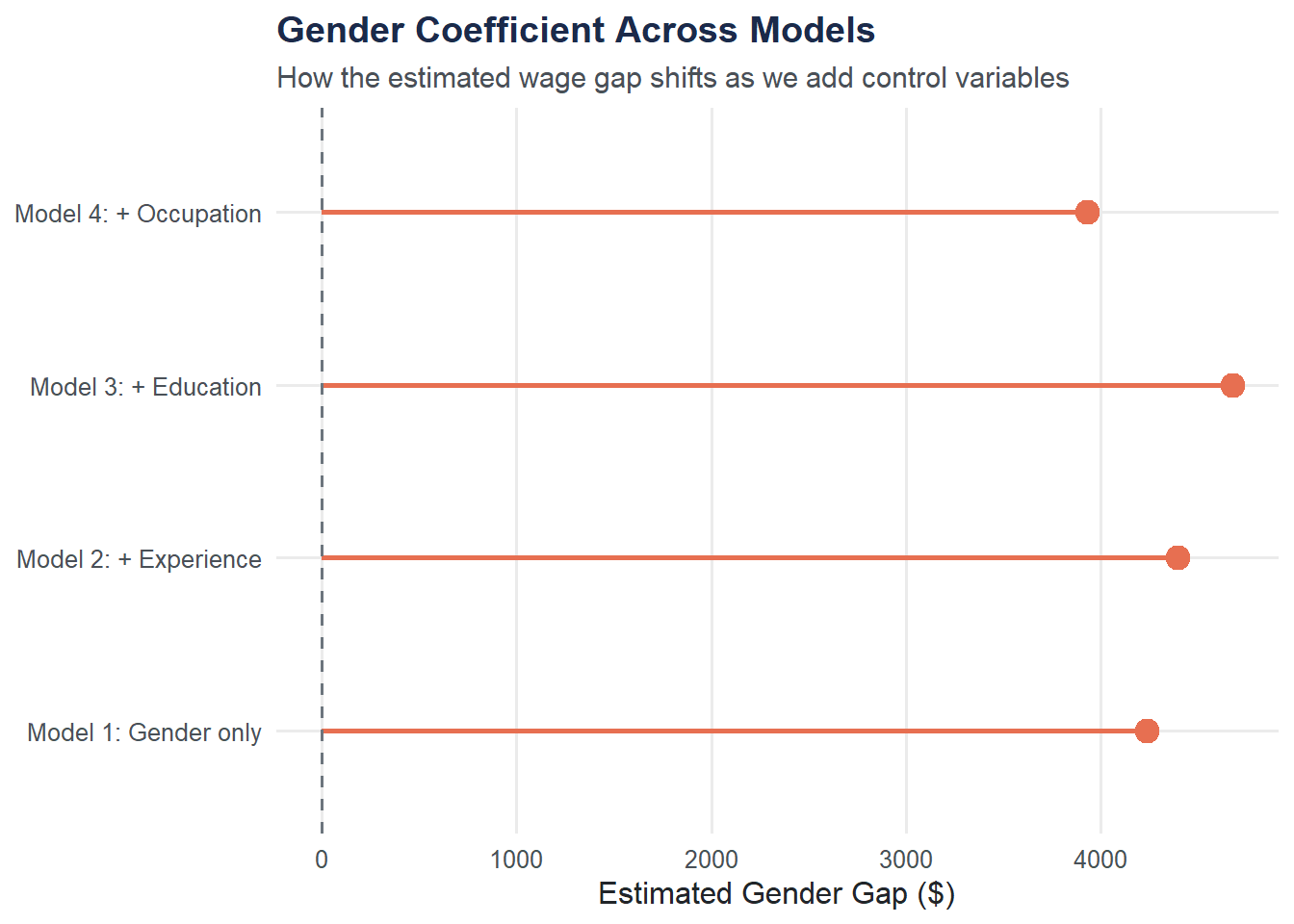
Multicollinearity Check: VIF
When predictors are highly correlated with each other, coefficient estimates become unstable. The Variance Inflation Factor (VIF) quantifies this. A VIF above 5 (some use 10) is cause for concern.
library(car)
vif(model4)
GVIF Df GVIF^(1/(2*Df))
gender 1.227183 1 1.107783
years_experience 1.188824 1 1.090332
education_years 1.910504 1 1.382210
occupation 2.056254 5 1.074751If any VIF is large, consider whether two predictors are measuring essentially the same thing.
Coefficient Plot: Full Model
A dot-and-whisker plot displays all coefficients from Model 4 with their 95% confidence intervals. Coefficients whose intervals do not cross zero are statistically significant.
coef_df <- broom::tidy(model4, conf.int = TRUE) |>
  filter(term != "(Intercept)")

ggplot(coef_df, aes(x = estimate, y = reorder(term, estimate))) +
  geom_vline(xintercept = 0, linetype = "dashed", color = moe_colors$slate) +
  geom_errorbarh(aes(xmin = conf.low, xmax = conf.high),
                 height = 0.2, color = moe_colors$navy) +
  geom_point(size = 3, color = moe_colors$coral) +
  labs(
    title = "Model 4: Coefficient Estimates",
    subtitle = "Bars show 95% confidence intervals; dashed line = zero",
    x = "Coefficient Estimate ($)",
    y = NULL
  ) +
  theme_moe()
Warning: `geom_errobarh()` was deprecated in ggplot2 4.0.0.
ℹ Please use the `orientation` argument of `geom_errorbar()` instead.`height` was translated to `width`.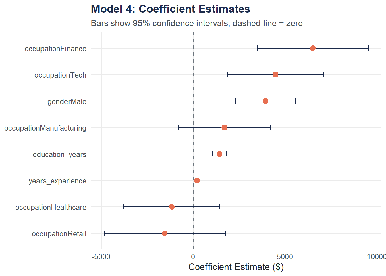
Try It Yourself
Expand the model. Add
regionandunion_memberto Model 4:lm(salary ~ gender + years_experience + education_years + occupation + region + union_member, data = wages). Does the gender coefficient change further? Does R-squared improve substantially?Residual check. Create a residual plot for the full model (fitted values on the x-axis, residuals on the y-axis). Are there any patterns or signs of non-constant variance (heteroscedasticity)?