# Loads tidyverse, book color palette, and theme_moe()
# Download _common.R from the Datasets page if running locally
source("_common.R")Chapter 8: Hypothesis Testing
Overview
Hypothesis testing is a formal framework for deciding whether observed patterns are real or due to chance. In this walkthrough, we analyze data from a landmark study on racial discrimination in hiring: researchers sent fictitious resumes to real job postings, randomly assigning either a stereotypically white or Black name. The callback rates reveal whether name — a proxy for perceived race — affected who got called back. This walkthrough accompanies Chapter 8 of Margin of Error.
Setup
Load and Explore the Data
The dataset contains 4,870 fictitious resume submissions. The key variable is callback — whether the employer called back.
resumes <- read_csv("data/resume-callbacks.csv")Rows: 4870 Columns: 7
── Column specification ────────────────────────────────────────────────────────
Delimiter: ","
chr (5): name_type, gender, resume_quality, education, callback
dbl (2): resume_id, years_experience
ℹ Use `spec()` to retrieve the full column specification for this data.
ℹ Specify the column types or set `show_col_types = FALSE` to quiet this message.glimpse(resumes)Rows: 4,870
Columns: 7
$ resume_id <dbl> 1, 2, 3, 4, 5, 6, 7, 8, 9, 10, 11, 12, 13, 14, 15, 16…
$ name_type <chr> "White-sounding", "White-sounding", "Black-sounding",…
$ gender <chr> "Female", "Female", "Female", "Female", "Female", "Ma…
$ resume_quality <chr> "Low", "High", "Low", "High", "High", "Low", "High", …
$ years_experience <dbl> 6, 6, 6, 6, 22, 6, 5, 21, 3, 6, 8, 8, 4, 4, 5, 4, 5, …
$ education <chr> "Bachelor", "High School", "Bachelor", "High School",…
$ callback <chr> "No", "No", "No", "No", "No", "No", "No", "No", "No",…resumes |>
count(name_type, callback) |>
arrange(name_type, callback)# A tibble: 4 × 3
name_type callback n
<chr> <chr> <int>
1 Black-sounding No 2278
2 Black-sounding Yes 157
3 White-sounding No 2200
4 White-sounding Yes 235Callback Rates by Name Type
The central question: do callback rates differ by name type?
callback_summary <- resumes |>
  group_by(name_type) |>
  summarize(
    n = n(),
    callbacks = sum(callback == "Yes"),
    callback_rate = mean(callback == "Yes")
  )

callback_summary
# A tibble: 2 × 4
name_type n callbacks callback_rate
<chr> <int> <int> <dbl>
1 Black-sounding 2435 157 0.0645
2 White-sounding 2435 235 0.0965There is a visible gap. But is it statistically significant, or could it have arisen by chance?
Two-Sample Proportion Test
We test \(H_0\): the callback rate is the same for both name types vs. \(H_a\): the rates differ.
# prop.test expects: c(successes_group1, successes_group2), c(n1, n2)
prop_result <- prop.test(
  x = callback_summary$callbacks,
  n = callback_summary$n
)

prop_result
    2-sample test for equality of proportions with continuity correction

data:  callback_summary$callbacks out of callback_summary$n
X-squared = 16.449, df = 1, p-value = 4.998e-05
alternative hypothesis: two.sided
95 percent confidence interval:
 -0.04769866 -0.01636705
sample estimates:
    prop 1     prop 2
0.06447639 0.09650924 cat("Difference in proportions:",
round(diff(callback_summary$callback_rate), 4), "\n")Difference in proportions: 0.032 cat("Chi-squared statistic:", round(prop_result$statistic, 2), "\n")Chi-squared statistic: 16.45 cat("p-value:", format.pval(prop_result$p.value, digits = 4), "\n")p-value: 4.998e-05 cat("95% CI for difference:", round(prop_result$conf.int[1], 4), "to",
round(prop_result$conf.int[2], 4), "\n")95% CI for difference: -0.0477 to -0.0164 Two-Sample t-Test on Years of Experience
The resumes were randomly assigned names, so years of experience should not differ by name type. Let’s verify with a t-test.
t_result <- t.test(years_experience ~ name_type, data = resumes)
t_result
    Welch Two Sample t-test

data:  years_experience by name_type
t = -0.18462, df = 4867.1, p-value = 0.8535
alternative hypothesis: true difference in means between group Black-sounding and group White-sounding is not equal to 0
95 percent confidence interval:
 -0.3101545  0.2567664
sample estimates:
mean in group Black-sounding mean in group White-sounding
7.829569 7.856263 cat("Mean experience (Black names):",
round(t_result$estimate[1], 2), "\n")Mean experience (Black names): 7.83 cat("Mean experience (White names):",
round(t_result$estimate[2], 2), "\n")Mean experience (White names): 7.86 cat("p-value:", round(t_result$p.value, 4), "\n")p-value: 0.8535 As expected, there is no significant difference — the randomization worked.
Chi-Square Test of Independence
The chi-square test is another way to test whether callback and name type are independent.
chi_table <- table(resumes$callback, resumes$name_type)
chi_result <- chisq.test(chi_table)
chi_result
    Pearson's Chi-squared test with Yates' continuity correction

data:  chi_table
X-squared = 16.449, df = 1, p-value = 4.998e-05cat("Chi-squared statistic:", round(chi_result$statistic, 2), "\n")Chi-squared statistic: 16.45 cat("Degrees of freedom:", chi_result$parameter, "\n")Degrees of freedom: 1 cat("p-value:", format.pval(chi_result$p.value, digits = 4), "\n")p-value: 4.998e-05 The chi-square p-value is consistent with the proportion test above.
The Danger of P-Hacking
P-hacking is the practice of testing many hypotheses and reporting only the significant ones. If you test 20 unrelated variables at the 5% level, you expect about 1 false positive by pure chance.
set.seed(42)
n_obs <- 200
n_tests <- 20

# Generate a binary outcome and 20 random predictors (no true relationship)
outcome <- sample(c("Yes", "No"), n_obs, replace = TRUE)
random_vars <- map(1:n_tests, ~ rnorm(n_obs))

# Test each predictor against the outcome using a t-test
p_values <- map_dbl(random_vars, function(x) {
  t.test(x ~ outcome)$p.value
})

phack_data <- tibble(
  test_number = 1:n_tests,
  p_value = p_values,
  significant = p_value < 0.05
)

ggplot(phack_data, aes(x = factor(test_number), y = p_value,
                       fill = significant)) +
  geom_col(width = 0.7) +
  geom_hline(yintercept = 0.05, linetype = "dashed",
             color = moe_colors$coral, linewidth = 0.8) +
  scale_fill_manual(
    values = c("TRUE" = moe_colors$coral, "FALSE" = moe_colors$teal),
    labels = c("TRUE" = "p < 0.05 (false positive)", "FALSE" = "Not significant")
  ) +
  annotate("text", x = 18, y = 0.07, label = "alpha = 0.05",
           color = moe_colors$coral, fontface = "italic", size = 3.5) +
  labs(
    title = "P-Hacking: Testing 20 Random Variables",
    subtitle = "None of these variables are truly related to the outcome",
    x = "Test number",
    y = "p-value",
    fill = NULL
  ) +
  theme_moe()

cat("Number of 'significant' results:", sum(phack_data$significant),
    "out of", n_tests, "\n")
Number of 'significant' results: 2 out of 20 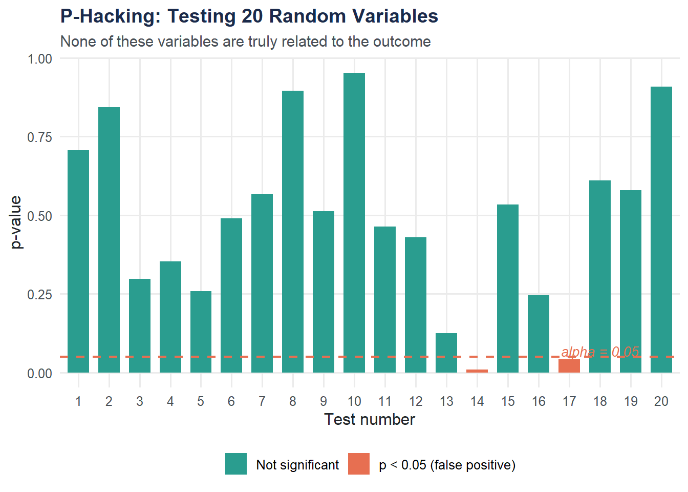
Any “significant” result here is a false positive — there is no real relationship. This is why multiple testing corrections matter.
Visualization: Callback Rates by Name Type and Resume Quality
rate_by_quality <- resumes |>
  group_by(name_type, resume_quality) |>
  summarize(callback_rate = mean(callback == "Yes"), .groups = "drop")

ggplot(rate_by_quality, aes(x = resume_quality, y = callback_rate,
                            fill = name_type)) +
  geom_col(position = "dodge", width = 0.7) +
  scale_fill_moe() +
  scale_y_continuous(labels = scales::percent_format()) +
  labs(
    title = "Callback Rates by Name Type and Resume Quality",
    subtitle = "The gap persists across both quality levels",
    x = "Resume Quality",
    y = "Callback Rate",
    fill = "Name Type"
  ) +
  theme_moe()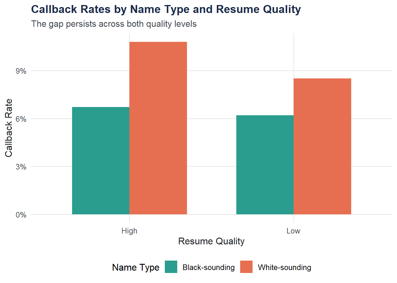
The discrimination gap is visible at both quality levels. Higher-quality resumes get more callbacks overall, but the disparity between name types persists.
Try It Yourself
Does callback rate differ by gender? Use
prop.test()orchisq.test()to test whether callback rates differ between male and female applicants. What do you find? Does gender discrimination appear in these data?How common are false positives? Run the p-hacking simulation 100 times (each time testing 20 random variables). In what fraction of the 100 runs do you find at least one “significant” result? The theoretical answer is \(1 - (1 - 0.05)^{20} \approx 0.64\). Does your simulation match?